8 Reporting

I love deadlines. I love the whooshing noise they make as they go by.¹

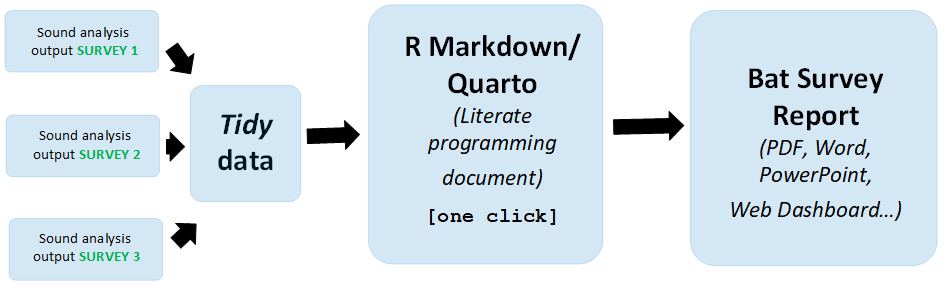
Transforming sound analysis data into a comprehensive bat survey report has never been easier — a simple mouse click can complete the entire process Figure 8.1. This streamlined reporting is made possible through literate programming, as introduced by Donald Knuth (Knuth 1984). In literate programming, code and descriptive writing seamlessly coexist within the same document, allowing for simultaneous execution and explanation of data analysis. This approach not only enhances efficiency but also provides a clear and integrated workflow. Generate a Word report with just one click Section 8.3.1, or effortlessly create a PowerPoint presentation in the same manner Section 8.3.2. Literate programming empowers bat data scientists with a remarkably straightforward and efficient reporting experience.

8.1 Why Use Literate Programming in Bat Data Science?

8.1.1 Advantages of this Approach:

Workflow Efficiency:
- Reduction of Copy-Paste: Minimizes or eliminates manual copy-pasting activities.
- Effortless Report Creation: Reports can be generated with a single click, accommodating new data or updates seamlessly.
- Time Savings: Significantly reduces the time and effort needed to produce reports, often by several orders of magnitude.
Reproducibility:
- Personal and Collaborative Reproducibility: The report can be easily reproduced by both the author and collaborators, proving valuable when revisiting a project after an extended period².
Open Source Approach:
- Accessible Editing: The Quarto or R Markdown file, constituting the literate program document, is plain text and can be edited using any text editor. However, using integrated development environments like RStudio is recommended³.
- Free Software Tools: The software tools⁴ used to interpret the literate program document and generate reports in various formats (Word, PDF, PowerPoint, or Dashboards) are open source and freely available for use.

8.1.2 Any Drawbacks?

Coding Skills Requirement:
- Literate Programming Document: Writing the literate program document requires coding skills. Section 9.4 shows how Large Language Models, such as ChatGPT can assist with coding.
- Coding Skills of the Ecologist: Coding skills in ecology are still evolving, though many universities are incorporating coding into their ecological courses. It’s important to note that minimal to no coding skills are necessary for rendering the literate programming document into the final report.

8.2 Document Structure for Literate Programming

Literate programming combines code and documentation in a single document, enhancing clarity and understanding. The structure typically includes:

YAML Header: see Section 8.2.1
- Positioned at the document’s beginning.
- Specifies metadata, settings, and document properties.
Markdown Body Text: see Section 8.2.2
- Written in Markdown for easy readability.
- Includes narrative text, explanations, and context.
Code Chunks: see Section 8.2.3
- Embedded code snippets or blocks.
- Can be executed to generate results directly within the document.
Citations with BibTeX: see Section 8.2.4
- For referencing external sources.
Equations: see Section 8.2.5
- Mathematical expressions written in LaTeX within Markdown.

Literate programming promotes a holistic approach to document creation, emphasizing the seamless integration of narrative, code, and documentation to enhance both understanding and maintainability.

8.2.1 YAML

YAML itself stands for Yet Another Markup Language, but in Quarto and RMarkdown, it simply refers to the front matter section at the beginning of your document. The YAML header is used to set metadata and configure various options for the document. The YAML headers provide a way to customize the appearance and behaviour of the document, including options for output formats, bibliographies, and more. Adjustments can be made based on the specific requirements of your document and the desired output format. Common YAML fields and their usage, along with examples for both Quarto and RMarkdown are shown below.

8.2.1.1 YAML Header in RMarkdown:

---
title: "My Document"
author: "John Doe"
date: "2024-01-29"
output:
  pdf_document:
    toc: true
    number_sections: true
    highlight: tango
bibliography: myreferences.bib
---

# Introduction

This is a simple RMarkdown document.

Explanation:

title: The title of the document.
author: The author(s) of the document.
date: The date of the document.
output: Specifies the output format and related options. In this example, it’s set to create a PDF document with a table of contents, numbered sections, and syntax highlighting using the ‘tango’ style.
bibliography: Specifies the BibTeX file for managing references.

8.2.1.2 YAML Header in Quarto:

---
title: "My Document"
authors:
  - name: John Doe
    affiliation: University of Quarto
date: "2024-01-29"
output:
  pdf_document:
    toc: true
    number_sections: true
    highlight: tango
bibliography:
  - myreferences.bib
---

# Introduction

This is a simple Quarto document.

Explanation:

title: The title of the document.
authors: A list of authors with optional affiliations⁵.
date: The date of the document.
output: Specifies the output format and related options. Similar to RMarkdown, this example is set to create a PDF document with a table of contents, numbered sections, and syntax highlighting using the ‘tango’ style.
bibliography: Specifies the BibTeX file for managing references; see Section 8.2.4.

8.2.2 Markdown

Markdown is a lightweight markup language that is easy to read and write. It’s commonly used for formatting text on the web, including in platforms like GitHub, Reddit, and various blogging systems. Here’s a basic guide to Markdown formatting:

8.2.2.1 Headers

# Heading 1
## Heading 2
### Heading 3
#### Heading 4
##### Heading 5
###### Heading 6

8.2.2.2 Emphasis

*Italic text* or _Italic text_
**Bold text** or __Bold text__
**_Combined emphasis_**
~~Strikethrough~~

Italic text
Bold text
Combined emphasis
~~Strikethrough~~

8.2.2.3 Lists

Unordered List:

- Item 1
- Item 2
  - Subitem 2.1
  - Subitem 2.2
* Item 3

Item 1
Item 2
- Subitem 2.1
- Subitem 2.2
Item 3

Ordered List:

1. First item
2. Second item
   1. Subitem 2.1
   2. Subitem 2.2
3. Third item

First item
Second item
1. Subitem 2.1
2. Subitem 2.2
Third item

8.2.2.4 Links

[Link Text](https://www.bats.org.uk/)

Link Text

8.2.2.5 Images

![image text](images/R_logo.png)

8.2.2.6 Blockquotes

> This is a blockquote.
> You can add multiple lines.

This is a blockquote. You can add multiple lines.

8.2.2.7 Inline Code

Use backticks for inline code: this answer is 42.

Use backticks for inline code: this answer is 42.

Inserting chunks of code is described in Section 8.2.3.

8.2.2.8 Tables

| Header 1 | Header 2 |
|----------|----------|
| Row 1, Col 1 | Row 1, Col 2 |
| Row 2, Col 1 | Row 2, Col 2 |

Header 1	Header 2
Row 1, Col 1	Row 1, Col 2
Row 2, Col 1	Row 2, Col 2

8.2.2.9 Task Lists

- [x] Task 1
- [ ] Task 2
- [ ] Task 3

Task 1
Task 2
Task 3

8.2.3 Code Chunks

Both Quarto and RMarkdown use code chunks to integrate executable code within their documents. These chunks allow you to seamlessly combine narrative text with data analysis, visualization, and other computational tasks.

Structure:

A code chunk starts and ends with three backticks ```, followed by optional information within curly braces. This information specifies the language ({r}, {python}, etc.) and other options for execution and output.

Show the code

# This is a code chunk
print("Hello, world!")

[1] "Hello, world!"

Output Display:

There are various ways to display the output of code chunks:

Inline Code: For short snippets, use backticks (`) around the code to display it inline with the text see Section 8.2.2.7.
Print Output: The default behavior is to print the output of the code directly below the chunk; this can be suppressed etc…
Plot Output: If the code generates a plot, it will be embedded below the chunk by default.
Formatted Output:
- RMarkdown options like eval=FALSE, echo=FALSE, and fig.cap= control how code, results, and captions are displayed.
- Quarto options like eval: false, echo: false, and fig.cap: control how code, results, and captions are displayed.

Additional Options:

Output format: Specify output=kable() for tables, output=html() for formatted HTML output, or other formats depending on the language.
Chunk labels: Assign unique labels to chunks for referencing or cross-linking within the document.
Chunk options: Customize output behavior with advanced options like cache=TRUE, warning=FALSE, and more.

Key Differences:

While both tools share similar concepts, there are some differences:

Engine: Quarto supports various languages through different engines, while RMarkdown primarily focuses on R.
Output formats: Quarto and RMarkdown offer a wider range of output formats besides HTML, like PDF, docx, and more.
Features: Quarto provides additional features like interactive elements and document styling options.

The specific features and options may vary depending on the chosen language and rendering engine. Refer to the respective documentation for comprehensive details.

8.2.4 Citations

8.2.4.1 BibTeX File and its Use in Citations:

BibTeX is a reference management tool that is widely used in conjunction with LaTeX, a typesetting system commonly used for the production of scientific and mathematical documents due to its excellent handling of complex structures like equations and references.

A BibTeX file is a plain text file (.bib) that contains bibliographic entries. Each entry in the file corresponds to a reference (e.g., a book, article, or conference paper). Each entry has specific fields (e.g., author, title, journal, year) that contain information about the reference.

A sample BibTeX entry might look like this:

@article{Author2020,
  author    = {Author, A.},
  title     = {Title of the Article},
  journal   = {Journal Name},
  year      = {2020},
  volume    = {10},
  number    = {2},
  pages     = {123-145},
}

The @article indicates the type of reference (in this case, an article), and the unique key (Author2020) is used to cite this reference in a LaTeX document.

8.2.4.2 Software for Managing Citations with BibTeX:

Several free software tools are available for managing citations through BibTeX files. Here are a few examples:

JabRef: An open-source reference manager with advanced features and an intuitive interface.
Zotero: While primarily a browser extension, Zotero also supports BibTeX export. It’s a versatile tool for managing references, collecting web content, and generating citations.
Mendeley: Mendeley is a reference manager and academic social network. It allows you to organize your references and generate BibTeX files.
BibDesk: BibDesk is a BibTeX editor for macOS, providing a simple interface for managing references.

8.2.4.3 Referencing Citations in Quarto or RMarkdown Document:

If you’re working with Quarto or RMarkdown documents, you can include citations using the cite syntax.

An example using RMarkdown:


---
title: "My Document"
output: pdf_document
bibliography: myreferences.bib
---

# Introduction

This is some text that needs a citation [@Author2020].

# References

In this example, the bibliography field specifies the BibTeX file containing your references. The [@Author2020] syntax is used to cite the reference with the key Author2020.

For Quarto, the syntax is similar:

---
title: "My Document"
bibliography:
  - myreferences.bib
---

# Introduction

This is some text that needs a citation [@Author2020].

# References

Make sure to replace myreferences.bib with the actual filename of your BibTeX file and Author2020 with the correct citation key from your file.

8.2.5 Mathematical Expressions

LaTeX math syntax provides a powerful and flexible way to create mathematical equations and expressions. The examples below showcase the versatility of LaTeX math syntax in expressing a wide range of mathematical concepts and structures. The syntax allows for precise and professional-looking mathematical typesetting, making it a standard choice in academic and scientific writing. A more complete guide to LaTeX mathematical expressions can be found here

8.2.5.1 Basic Math Operations:

$a^2 + b^2 = c^2$

This equation represents the Pythagorean theorem:

\(a^2 + b^2 = c^2\)

8.2.5.2 Fractions and Roots:


$\frac{1}{\sqrt{2}} \times \frac{\pi}{2}$

This equation combines fractions and square roots:

\(\frac{1}{\sqrt{2}} \times \frac{\pi}{2}\)

8.2.5.3 Greek Letters and Summation:

$\sum_{i=1}^{n} \alpha_i \cdot \beta_i$

This equation involves Greek letters and a summation:

\(\sum_{i=1}^{n} \alpha_i \cdot \beta_i\)

8.2.5.4 Integrals:

$\int_{0}^{\infty} e^{-x^2} \, dx$

This equation represents a Gaussian integral:

\(\int_{0}^{\infty} e^{-x^2} \, dx\)

8.2.5.5 Matrices:

$\begin{bmatrix}
1 & 2 & 3 \\
4 & 5 & 6 \\
7 & 8 & 9
\end{bmatrix}$

This creates a 3x3 matrix:

\(\begin{bmatrix} 1 & 2 & 3 \\ 4 & 5 & 6 \\ 7 & 8 & 9 \end{bmatrix}\)

8.2.5.6 Equations with Alignments:

$\begin{align*}
2x + 3y &= 8 \\
4x - 2y &= 6
\end{align*}$

This represents a system of linear equations:

\(\begin{align*} 2x + 3y &= 8 \\ 4x - 2y &= 6 \end{align*}\)

8.2.5.7 Complex Equations:

$f(x) = \frac{1}{2\pi i} \oint_C \frac{f(z)}{z-z_0} \, dz$

This involves a complex contour integral:

\(f(x) = \frac{1}{2\pi i} \oint_C \frac{f(z)}{z-z_0} \, dz\)

8.3 Example Bat Reports

8.3.1 Microsoft Word

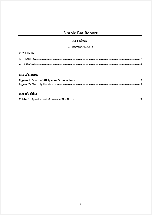
The complete R Markdown text (the .Rmd file) that produces a simple bat report from the statics tidy data⁶ is shown below; it can be copied to the clip board and rendered (knitted) into the Word report illustrated in Figure 8.2.

---
title: "Simple Bat Report"
output: 
  officedown::rdocx_document: default
date: "23 July, 2024"
author: "An Ecologist"
---

```{r include=FALSE}
library(knitr)
library(tidyverse)
library(iBats)
library(ggrepel)
library(broman)
library(flextable)
library(officer)
library(officedown)
library(treemapify)
library(ggthemes) 

knitr::opts_chunk$set(echo = FALSE, warnings = FALSE, message = FALSE)
knitr::opts_chunk$set(fig.cap = TRUE)

# A vector used to give the species a specific colour in the graphic; the colours
# can be changed and other species added.
bat_colours_sci <- c(
  "Barbastella barbastellus" = "#1f78b4",
  "Myotis alcathoe" = "#a52a2a",
  "Myotis bechsteinii" = "#7fff00",
  "Myotis brandtii" = "#b2df8a",
  "Myotis mystacinus" = "#6a3d9a",
  "Myotis nattereri" = "#ff7f00",
  "Myotis daubentonii" = "#a6cee3",
  "Myotis spp." = "#bcee68",
  "Plecotus auritus" = "#8b0000",
  "Plecotus spp." = "#8b0000",
  "Plecotus austriacus" = "#000000",
  "Pipistrellus pipistrellus" = "#ffff99",
  "Pipistrellus nathusii" = "#8a2be2",
  "Pipistrellus pygmaeus" = "#b15928",
  "Pipistrellus spp." = "#fdbf6f",
  "Rhinolophus ferrumequinum" = "#e31a1c",
  "Rhinolophus hipposideros" = "#33a02c",
  "Nyctalus noctula" = "#cab2d6",
  "Nyctalus leisleri" = "#fb9a99",
  "Nyctalus spp." = "#eee8cd",
  "Eptesicus serotinus" = "#008b8b"
)
```

__CONTENTS__
<!---BLOCK_TOC--->
__List of Figures__
<!---BLOCK_TOC{seq_id: 'fig'}--->
__List of Tables__
<!---BLOCK_TOC{seq_id: 'tab'}--->

```{r include=FALSE}
##### Load your TIDY bat data here:
# TidyBatData <- read_csv("YourTidyData.csv", col_names = TRUE)

# Tidy bat data - example data from the iBats package
TidyBatData <- statics
```

\newpage
# TABLES

The simplest form of aggregation is a count of bats[^1]; as shown in Table \@ref(tab:table01)
[^1]: note:- in this case it is a count of bat passes

```{r tab.id="table01", tab.cap="Species and Number of Bat Passes"}
TidyBatData %>%
  group_by(Species) %>% 
  count() %>% 
  #arrange descending
  arrange(desc(n)) %>% 
  # rename n as count
  rename(`Bat Species` = Species, Count = n) %>% 
  # so table is produced with individual species on one row
  ungroup() %>% 
  flextable() %>%
  width(j = 1, width = 2.5) %>%
  italic(j = 1, italic = TRUE, part = "body") %>%
  bg(bg = "black", part = "header") %>%
  color(color = "white", part = "header")
```

\newpage
# FIGURES  

Figure \@ref(fig:graph01) shows the count of all the species observations as a dot chart and Figure \@ref(fig:graph02) shows a treemap of monthly bat pass activity.

```{r graph01, fig.cap="Count of All Species Observations", fig.height=7, fig.width=6}

g_data <- TidyBatData %>% 
group_by(Species) %>% 
count() %>% 
mutate(total = add_commas(n),
       label = stringr::str_c(Species, ": ", total))
  
graph_bat_colours <- iBats::bat_colours(g_data$Species, colour_vector = bat_colours_sci)

p <- ggplot(g_data, aes(y = reorder(Species, n), x = n, fill = Species)) +
  geom_point(colour = "black", size = 5) +
  geom_label_repel(data = g_data, aes(label = label),
                   nudge_y = -0.25,
                   nudge_x = ifelse(g_data$n < 100, 0.33, -0.33),
                   alpha = 0.7) +
  scale_fill_manual(values = graph_bat_colours) +
  scale_x_log10(sec.axis = dup_axis()) +
  annotation_logticks(sides = "tb") +
  labs(x = "Bat Observations (Number of Passes)",
       caption = "Note: Log scale used") +
  theme_bw() + 
  theme(legend.position = "none", 
        panel.grid.major = element_blank(), 
        panel.grid.minor = element_blank(),
        axis.text.x = element_text(size=12, face="bold"), 
        axis.text.y = element_blank(), 
        axis.ticks.y = element_blank(),
        strip.text = element_text(size=12, face="bold", colour = "white"), 
        axis.title.x = element_text(size=12, face="bold"), 
        axis.title.y = element_blank())

p
```

\newpage
```{r graph02, fig.cap="Monthly Bat Activity", fig.height=7, fig.width=6}

# Add data and time information to the iBats statics bat survey data set using the iBats::date_time_info
statics_plus <- iBats::date_time_info(statics)

graph_data <- statics_plus %>%
  group_by(Species, Month) %>%
  tally()

ggplot(graph_data, aes(area = n, fill = Month, label = Species, subgroup = Month)) +
  scale_fill_tableau(palette = "Tableau 10") + #
  geom_treemap(colour = "white", size = 2, alpha = 0.9) +
  geom_treemap_subgroup_border(colour = "black", size = 5, alpha = 0.9) +
  geom_treemap_subgroup_text(place = "centre", grow = T, alpha = 0.9, colour = "grey20", min.size = 0) +
  geom_treemap_text(colour = "grey90", place = "topleft", fontface = "italic", reflow = T, min.size = 0, alpha = 0.9) +
  theme_bw() +
  theme(legend.position = "none") # No legend
```

The three page Word report shown in Figure 8.2 is a rudimentary example; it could be expanded to include any of the tables and graphs shown on these web pages. The .Rmd file is rendered into a Microsoft Word document; this is a convenient file format easily allowing further editing by others in the survey team. The simple report in Figure 8.2 has a tables of contents and cross referencing it can also be rendered directly into the house/company style by specifying a reference_docx file⁷.

8.3.2 PowerPoint

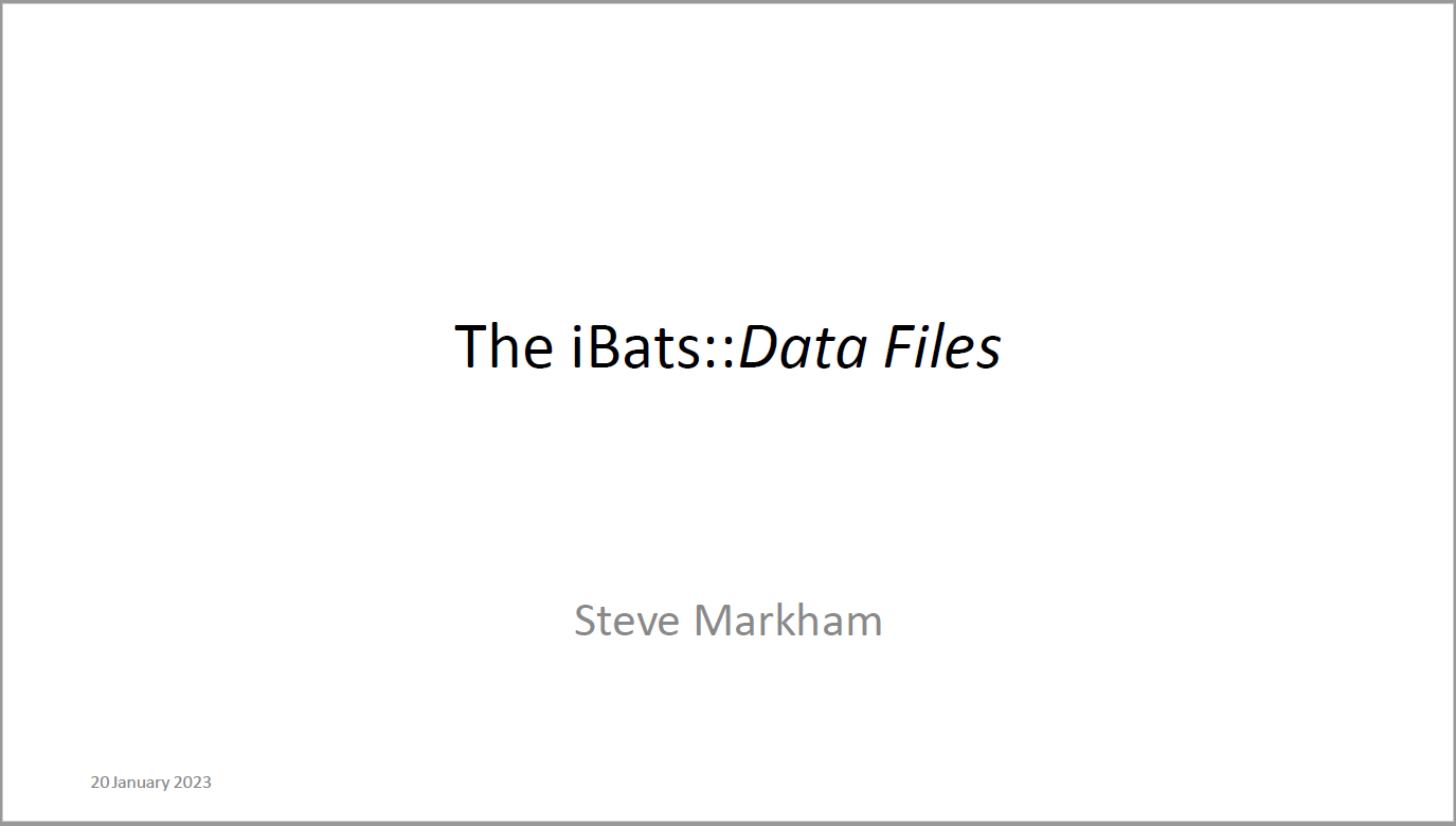
The R Markdown text (the .Rmd file) that produces a PowerPoint presentation on the data files in the iBats package is shown below; it can be copied to the clip board and rendered (knitted) into the PowerPoint presentation illustrated in Figure 8.3.

---
date: "23 July 2024"
author: "Steve Markham"
title: "The iBats::_Data Files_"
output: 
  officedown::rpptx_document
---

```{r setup, include=FALSE}
knitr::opts_chunk$set(echo = FALSE, warnings = FALSE, message = FALSE)

library(officedown)
library(ggplot2)
library(rvg)
library(tidyverse)
library(flextable)
library(officer)
library(sf)
library(ggspatial)
library(rnaturalearth)
library(rnaturalearthdata)
library(iBats)

```
## Annex II Species in `iBats::Statics`

```{r layout='Two Content', ph=officer::ph_location_left()}

# Add data and time information to the statics data using the iBats::date_time_info
statics_plus <- iBats::date_time_info(statics)

AnnexII <- c("Barbastella barbastellus", "Rhinolophus ferrumequinum", "Rhinolophus hipposideros")

table_border <- fp_border(color = "black", width = 1) # from library(officer)

statics_plus %>%
  filter(Species %in% AnnexII) %>%
  group_by(Species) %>%
  count() %>% 
  rename(`Bat Species` = Species, Count = n) %>%
  flextable(col_keys = colnames(.)) %>%
  italic(j = 1, italic = TRUE, part = "body") %>% 
  fontsize(part = "header", size = 12) %>%
  fontsize(part = "body", size = 12) %>%
  colformat_double(j = "Count", digits = 4, big.mark = ",") %>%
  width(j = 1, width = 2.5) %>%
  width(j = 2, width = 1) %>%
  border_inner_h(part = "body", border = table_border) %>%
  hline_bottom(part = "body", border = table_border) %>%
  bg(bg = "black", part = "header") %>%
  color(color = "white", part = "header")

```

```{r layout='Two Content', ph=officer::ph_location_right()}



graph_data <- statics_plus %>%
  filter(Species %in% AnnexII) %>%
  group_by(Species) %>%
  count() 

# colour values used by scale_fill_manual()
graph_bat_colours <- iBats::bat_colours_default(graph_data$Species)

mygg <- ggplot(graph_data, aes(x = "", y = n, fill = Species)) +
  geom_bar(width = 1, stat = "identity") +
  coord_polar(theta = "y") +
  scale_fill_manual(values = graph_bat_colours) +
  labs(
    y = "Bat Pass Observations (Nr)",
    fill = "Species"
  ) +
  theme_bw() +
  theme(
    legend.position = "bottom",
    legend.text = element_text(face = "italic"),
    axis.text.x = element_blank(),
    axis.text.y = element_blank(),
    axis.ticks = element_blank(),
    strip.text = element_blank(),
    axis.title.x = element_blank(),
    axis.title.y = element_blank(),
    panel.grid.major = element_blank(),
    panel.grid.minor = element_blank(),
    panel.background = element_blank(),
    panel.border = element_blank()
  ) +
  guides(fill=guide_legend(ncol =1))


dml(ggobj = mygg)

```

## Open Source Maps 

- Openstreet map
  - created by the online community
  - free to use (open license)
- Outline maps (counties, parish ...)
  - from the Office for National Statistics
  - used under the Open Government Licence
  - at a country scale the `rnaturalearth` package

## iBats::Lydford

```{r ph=officer::ph_location_left()}

#Outline maps countries
worldmap <- ne_countries(scale = 'medium', type = 'map_units',
                         returnclass = 'sf')

# GB only
GBcountires <- c("England", "Scotland", "Wales")
GB <- worldmap %>% 
  filter(name %in% GBcountires) %>% 
  select(geometry)

# Make location point for Mary Tavy Transect
MaryTavyLoc <- MaryTavy %>% 
  summarise(lat = median(`Latitude [WGS84]`),
            lon = median(`Longitude [WGS84]`)) %>% 
  st_as_sf(coords = c("lon", "lat")) %>% 
  st_set_crs(4326) %>% 
  # Convert coord reference system to British National Grid
  st_transform(crs = 27700)

p1 <- ggplot() +
  geom_sf(data = GB,
          linewidth = 0.25,
          colour = "black",
          fill = "#228b22") +
  geom_sf(data = MaryTavyLoc,
          shape = 23,
          size = 6,
          colour = "#00558e",
          fill = "#fab824") +
  theme_void() 

dml(ggobj = p1)

``` 

```{r ph=officer::ph_location_left(), eval = FALSE}

# Make location point for Mary Tavy Transect
MaryTavyLoc <- MaryTavy %>% 
  summarise(lat = median(`Latitude [WGS84]`),
            lon = median(`Longitude [WGS84]`)) %>% 
  st_as_sf(coords = c("lon", "lat")) %>% 
  st_set_crs(4326) %>% 
  # Convert coord reference system to British National Grid
  st_transform(crs = 27700)


# Load outline map
GB <- sf::st_read("maps/GeneralGB/CTYUA_Dec_2017_GCB_GB.shp", quiet = TRUE) %>% 
  filter(ctyua17nm == "Devon")

# Plot map and Location
p2 <- ggplot() +
  geom_sf(data = GB,
          linewidth = 0.25,
          colour = "#228b22",
          fill = "#98FB98") +
  geom_sf(data = MaryTavyLoc,
          shape = 23,
          size = 3,
          colour = "#00558e",
          fill = "#fab824") +
  labs(title = "Devon") +
  theme_void() +
  theme(title = element_text(colour = "#228b22", size = 14, face = "bold"))

dml(ggobj = p2)

``` 

```{r ph=officer::ph_location_right()}

spatial_data <- Lydford%>% 
  select(Species, longitude = Longitude, latitude = Latitude)

# default colour values used by scale_fill_manual() - scientific names - UK bats only
graph_bat_colours <- iBats::bat_colours_default(spatial_data$Species)

spatial_data <- st_as_sf(spatial_data, coords = c("longitude", "latitude"), 
                 crs = 4326)

p1 <- ggplot() +
  annotation_map_tile(type = "osm",  zoomin = -1, alpha = 0.5) +
  geom_sf(data = spatial_data, aes(fill = Species), shape = 21, alpha = 0.5, size = 4) +
  annotation_scale(location = "tl") +
  annotation_north_arrow(location = "bl", 
                         which_north = "true",
                         style = north_arrow_fancy_orienteering()) +
 # fixed_plot_aspect(ratio = 1) +
  coord_sf() +
  scale_fill_manual(values = graph_bat_colours) +
  scale_size_area(max_size = 12) +
  theme_void() +
  theme(legend.position = "right",
    axis.title.y = element_blank(),
    axis.title.x = element_blank(),
    axis.text.x = element_blank(),
    axis.text.y = element_blank(),
    axis.ticks = element_blank(),
    title = element_text(colour = "black", size = 14),
    legend.text = element_text(face = "italic"))

dml(ggobj = p1)

```

## iBats::TavyOak


- Time bats are active
- Better than a count?
- Foraging a large bubble?
- Commuting a small bubble?
- Modern bat detector data!

```{r ph=officer::ph_location_right()}
bat_colours_sci <- c(
  "Barbastella barbastellus" = "#1f78b4",
  "Myotis alcathoe" = "#a52a2a",
  "Myotis bechsteinii" = "#7fff00",
  "Myotis brandtii" = "#b2df8a",
  "Myotis mystacinus" = "#6a3d9a",
  "Myotis nattereri" = "#ff7f00",
  "Myotis daubentonii" = "#a6cee3",
  "Myotis spp." = "#bcee68",
  "Plecotus auritus" = "#8b0000",
  "Plecotus spp." = "#8b0000",
  "Plecotus austriacus" = "#000000",
  "Pipistrellus pipistrellus" = "#ffff99",
  "Pipistrellus nathusii" = "#8a2be2",
  "Pipistrellus pygmaeus" = "#b15928",
  "Pipistrellus spp." = "#fdbf6f",
  "Rhinolophus ferrumequinum" = "#e31a1c",
  "Rhinolophus hipposideros" = "#33a02c",
  "Nyctalus noctula" = "#cab2d6",
  "Nyctalus leisleri" = "#fb9a99",
  "Nyctalus spp." = "#eee8cd",
  "Eptesicus serotinus" = "#008b8b"
)

# graph anotation
graph_sunrise <- TavyOak$sunrise[1]
graph_sunset <- TavyOak$sunset[1]

# graph time limits x-axis
graph_limit1 <- TavyOak$sunset[1] - lubridate::hours(1)
graph_limit2 <- TavyOak$sunrise[1] + lubridate::hours(1)

# colour values used by scale_fill_manual()
graph_bat_colours <- iBats::bat_colours(TavyOak$Species, colour_vector = bat_colours_sci)

mygg <- ggplot(TavyOak, aes(y = 1, x = DateTime, fill = Species, size = bat_time)) +
  geom_jitter(shape = 21, alpha = 0.7) +
  geom_vline(
    xintercept = graph_sunset,
    colour = "brown1",
    linetype = "dashed",
    linewidth = 1,
    alpha = 0.8
  ) +
  geom_vline(
    xintercept = graph_sunrise,
    colour = "mediumblue",
    linetype = "dashed",
    linewidth = 1,
    alpha = 0.8
  ) +
  annotate("text",
    x = graph_sunset - lubridate::minutes(20),
    y = 1,
    label = "Sunset",
    color = "brown1",
    angle = 270
  ) +
  annotate("text",
    x = graph_sunrise + lubridate::minutes(20),
    y = 1,
    label = "Sunrise",
    color = "mediumblue",
    angle = 270
  ) +
  scale_fill_manual(values = graph_bat_colours) +
  scale_size_area(max_size = 12) +
  scale_x_datetime(
    date_labels = "%H:%M hrs",
    date_breaks = "1 hour",
    limits = c(graph_limit1, graph_limit2)
  ) +
  labs(
    fill = "Species",
    size = "Time Bat Was Present\n(seconds)",
    y = "For clarity activity is spread across the verstical scale"
  ) +
  theme_bw() +
  theme(
    legend.position = "right",
    panel.grid.major.x = element_line(),
    panel.grid.major.y = element_blank(),
    panel.grid.minor = element_blank(),
    axis.text.x = element_text(size = 10, angle = 270),
    axis.text.y = element_blank(),
    axis.ticks.y = element_blank(),
    strip.text = element_text(size = 12, face = "bold", colour = "white"),
    legend.text = element_text(face = "italic"),
    axis.title.x = element_blank(),
    axis.title.y = element_text(size = 10)
  )

dml(ggobj = mygg)

``` 

## iBats::MaryTavy

```{r layout='Title and Content', ph=officer::ph_location_type(type="body")}


###############################################################################
# MaryTavy is data directly exported from BatExplorer and requires tidying!####
###############################################################################

#### Combine the two Species columns into one ##################################
# Select Species column and remove (Species2nd & Species3rd)
data1 <- MaryTavy %>%
  select(-`Species 2nd Text`) %>% 
  rename(Species = `Species Text`)

# Select Species2nd column and remove (Species & Species3rd)
data2 <- MaryTavy %>%
  select(-`Species Text`) %>%
  filter(`Species 2nd Text` != "-") %>% # Remove blank rows
  rename(Species = `Species 2nd Text`) # Rename column

# Add the datasets together into one
MaryTavyTidying <- dplyr::bind_rows(data1, data2)
################################################################################


#### Calculate bat activity time and prepare to make spatial data #############
tidy_data <- MaryTavyTidying %>% 
  mutate(calls = `Calls [#]`,
         duration = `Mean Call Lenght [ms]`,
         span = `Mean Call Distance [ms]`,
         # Calculate BatActivityTime in seconds
         bat_time = calls * (duration + span) / 1000) %>% 
  select(Species, bat_time)

#Make species have common names
tidy_data$Species <- bat_common_default(tidy_data$Species)

# Aggregate data into Species and count
tidy_data %>%
  group_by(Species) %>% 
  summarise(bat_time = sum(bat_time)) %>% 
  arrange(desc(bat_time)) %>% 
  mutate(bat_time = round(bat_time, digits = 0),
         bat_time = lubridate::seconds_to_period(bat_time)) %>% 
  rename(`Bat Activity Time` = bat_time)

```

Douglas Adams, The Salmon of Doubt: Hitchhiking the Galaxy One Last Time; published posthumously (2002).↩︎
the exact same report can be reproduced if given access to the original data and Quarto®/RMarkdown literate programming document.↩︎
RStudio is now known as Posit https://posit.co/; and now embraces R and Python.↩︎
e.g. R https://www.r-project.org/, Python https://www.python.org/, R Markdown https://rmarkdown.rstudio.com/, Quarto® https://quarto.org/, RStudio https://posit.co/, Jupyter https://jupyter.org/.↩︎
The Quarto YAML can include more complex structures for authors and affiliations compared to RMarkdown.↩︎
From the iBats package.↩︎
More information on the production of Word documents and PowerPoint presentations from R and R Markdown is available from the work of David Gohel see https://ardata-fr.github.io/officeverse/index.html.↩︎