Statistical tests are undertaken to improve ecological understanding, separating the single from the noise. It enhances the ecological description when writing reports, making the report more evidenced based and therefore more robust. When the data is not clear, or there is too much data to see, good statistics brings comprehension. Then there is a tendency to perceive connections or meaningful patterns between unrelated or random things, termed apophenia; here statistical testing can demonstrate it is random or unrelated.
Before undertaking data analysis it is prudent to perform some exploration of the data. Data exploration will help identify potential problems in the data and assist in deciding what type of analysis to conduct.
Relationships among response and independent variables
Independence of the response variable.
7.2 Summary Statistics
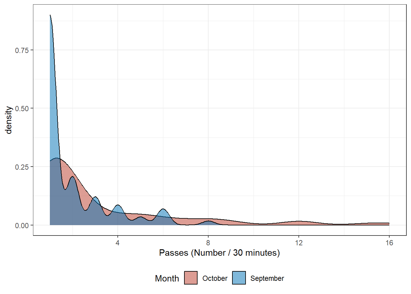
The Common Pipistrelle passes have been aggregated for every 30 minutes; Table 7.1 shows summary statistics for these bat passes during September and October. The statistics for September and October look similar and this is confirmed by the kernel density (Glossary B.2.4) plot shown in Figure 7.1.
Table 7.1: Summary Statistics for Common Pipistrelle Passes
Month
Min
Q1
Mean
Median
Q3
Max
sd
Nr
September
1
1
1.92
1
2
8
1.55
83
October
1
1
3.08
2
4
16
3.28
91
Where:
Min:- Minimum value.
Q1:- Lower quartile, or first quartile (Q1), the value under which 25% of data points are found when they are arranged in increasing order (Glossary B.3.1).
Mean:- Arithmetic mean of a dataset is the sum of all values divided by the total number of values.
Median:- The middle number; found by ordering all data points and picking out the one in the middle (or if there are two middle numbers, taking the mean of those two numbers).
Q3:- Upper quartile, or third quartile (Q3), is the value under which 75% of data points are found when arranged in increasing order (Glossary B.3.1).
Max:- Maximum value.
sd:- Standard deviation, a summary measure of the differences of each observation from the mean.
Figure 7.1: Comon Pipistrelle Passes September and October
7.3 Comparing Two Groups
Using the Wilcoxon signed rank test (Glossary B.5.1) we can decide, using a hypothesis test (Glossary B.5.3), whether the population distributions, summarised in Table 7.1 and Figure 7.1 are identical. An advantage of the Wilcoxon signed rank test is that it can be undertaken without assuming the data follows the normal distribution; the density plot in Figure 7.1 shows the data is unlikely to be normal. The two data samples for September and October need to be independent; the number of passes recorded separately in September and October are distinct populations where the passes do not affect each other.
It is assumed The survey effort (length of time the bat detectors where deployed and the locations are the same for both months)
Without assuming the data to have normal distribution, decide at .01 significance level (p < 0.01)1 if the observations of Common pipistrelle bats (every 30 minutes) for September and October have identical data distribution.
The null hypothesis H0: is that the common pipistrelle observation data for September and October are identical populations.
The alternate hypothesis H1: is that the common pipistrelle observation data of September and October are not identical populations.
To test the hypothesis, we apply the wilcox.test function to compare the independent samples.
Show the code
library(broom)mw <-wilcox.test(Passes ~ Month, data=Count30) #Tidy the out put into a tabletidy(mw) %>%gt() %>%tab_style(style =list(cell_fill(color ="black"),cell_text(color ="white", weight ="bold") ),locations =cells_column_labels(columns =c(everything()) ) )
Table 7.2: Summary Statistics for Common Pipistrell Passes
statistic
p.value
method
alternative
4533
0.0129358
Wilcoxon rank sum test with continuity correction
two.sided
Results from the the wilcox.test are shown in Table 7.2; as the p-value (Glossary B.5.4) turns out to be 0.0129358, and is not less than the .01 significance level2, we do not reject the null hypothesis. At .01 significance level (p < 0.01), we conclude that the common pipistrelle observation data for September and October are identical populations.
7.4 Comparing More Than Two Groups
7.4.1 An Obvious Difference
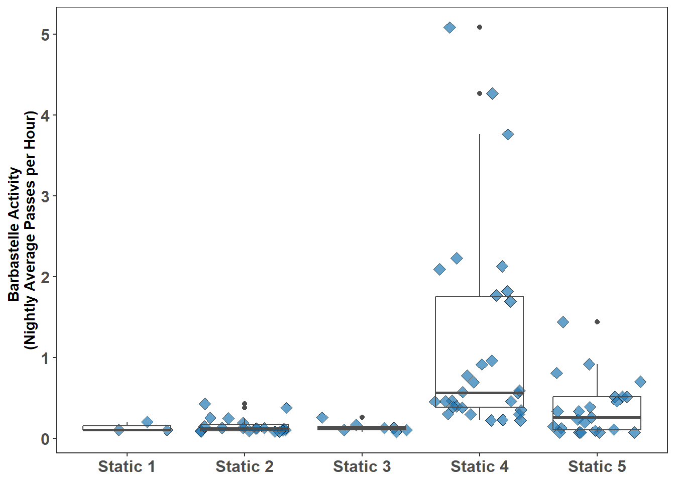
The statics data in the iBats package has some interesting Barbastelle (Barbastella barbastellus) bat activity, it would be interesting and aid our understanding if we compare the activity between static locations and see if they are significantly different.
Before undertaking any statistical test always visualise the data the statistical test is applied to; here the box plot is used (Glossary B.2.2). Figure 7.2 shows the Barbastelle recorded at several locations.
The average bat pass rate per hour can been calculated for each night and each static location using the formula shown in Equation 7.1:
Where: Batpasses = number of bat pass during the night at the location Nightlength = length of the night in decimal hours AverageActivity = average (mean) number of bat passes per hour for each night there was activity
Show the code
# Add data and time information to the statics data using the iBats::date_time_infostatics_plus <- iBats::date_time_info(statics)# Add sun and night time metrics to the statics data using the iBats::sun_night_metrics() function.statics_plus <- iBats::sun_night_metrics(statics_plus)graph_data <- statics_plus %>%filter(Species =="Barbastella barbastellus") %>%group_by(Description, Night, night_length_hr) %>%# count number of passes per night by species - makes coloumn "n""tally() %>%# calculate average bat passes per hour for each Night and speciesmutate(ave_act_per_hr = n / night_length_hr) %>%# Remove Night Length column from the Tableselect(-night_length_hr, -n) ggplot(graph_data, aes(y = ave_act_per_hr, x = Description)) +geom_jitter(fill ="#1f78b4", #Barbastelle colourcolour ="black", shape =23, alpha =0.7, size =3) +geom_boxplot(colour ="grey30", fill ="transparent") +labs(y ="Barbastelle Activity \n(Nightly Average Passes per Hour)") +theme_bw() +theme(legend.position ="none", # No legendaxis.text.x =element_text(size=12, face="bold"), axis.text.y =element_text(size=12,face="bold"), axis.title.y =element_text(face="bold"), axis.title.x =element_blank(), # no y title (just bat names)panel.grid.major =element_blank(), #remove grid linespanel.grid.minor =element_blank())
Figure 7.2: Barbastelle Activity at Each Static (Nightly Average Passes per Hour)
The comparison of locations is undertaken with the Kruskal-Wallis test (Glossary B.5.2). The Kruskal–Wallis test is a rank-based test that is similar to the Wilcoxon signed rank test but can be applied to one-way data with more than two groups. If there are just two locations the Wilcoxon signed rank test should be applied. The Kruskal–Wallis test may be used when there are only two samples, but the Wilcoxon signed rank test is more powerful for two samples and is preferred. Both tests assume that the observations are independent. The probability threshold for statistical significance, which should always be chosen before the test is undertaken, is: P < 0.05.
The Null Hypothesis: bat pass rates per hour are from distributions with the same median.
The Alternative Hypothesis: bat pass rates per hour are from distributions with a different median.
The function kruskal.test, from base R, is used to undertake the Kruskal-Wallis test. A rule of thumb for the Kruskal–Wallis test is each group, (in this case case the number of nightly average bats pace vales for each static location) must have a sample size of 5 or more.
Show the code
# Add data and time information to the statics data using the iBats::date_time_infostatics_plus <- iBats::date_time_info(statics)# Add sun and night time metrics to the statics data using the iBats::sun_night_metrics() function.statics_plus <- iBats::sun_night_metrics(statics_plus)test_data <- statics_plus %>%filter(Species =="Barbastella barbastellus") %>%group_by(Description, Night, night_length_hr) %>%# count number of passes per night by species - makes coloumn "n""tally() %>%# calculate average bat passes per hour for each Night and speciesmutate(ave_act_per_hr = n / night_length_hr) %>%# Remove Night Length column from the Tableselect(-night_length_hr, -n)# Check at least 2 locations and a minimum of 5 observations per location# Only do KW on locations with 5 or more observations# if just two locations do Mann Whitneycheck_data <- test_data %>%group_by(Description) %>%tally()# filter for Statics with more than 5 valuesStaticsWithPlus5 <- check_data %>%filter(n >=5) %>%pull(Description)test_data <- test_data %>%filter(Description %in% StaticsWithPlus5)# Extract the p-value from the kruskal.teststat_pvalue <-kruskal.test(ave_act_per_hr ~ Description, data = test_data)$p.value
With reference to Figure 7.2 there are several static locations where the activity can be compared, this is more than two locations, therefore the Kruskal-Wallis test is undertaken rather than the Mann-Whitney-Wilcoxon test. Location 1 with only three results is excluded from the test.
The Kruskal-Wallis test undertaken for the Barbastelle at the following static locations: Static 2, Static 3, Static 4, and Static 5 produced a P value (9.17e-08) less than the chosen threshold for statistical significance of 0.05; therefore the null hypothesis is rejected, activity between some static locations is likely to be different.
What the Kruskal-Wallis test does not indicate, is which static locations are different; to determine this we need to undertake post hoc testing, this can be undertaken with the Dunn’s Test (Glossary B.5.2).
Results of the Dunn’s test, performed after the Kruskal-Wallis test (post hoc), are shown in Table 7.3.
Show the code
df <-tibble(dunn_result$comparisons, dunn_result$P.adjusted)colnames(df) <-c("Comparison", "P.adj")resultsTable <- df %>%filter(P.adj <0.05) %>%select(`Locations with a significant difference (P<0.05)`= Comparison, `adjusted P `= P.adj)resultsTable %>%flextable(col_keys =colnames(.)) %>%fontsize(part ="header", size =12) %>%fontsize(part ="body", size =12) %>%bold(part ="header") %>%autofit(add_w =0.1, add_h =0.1) %>%bg(bg ="black", part ="header") %>%color(color ="white", part ="header") %>%align(align ="center", part ="header") %>%align(j =2, align ="right", part ="body") %>%bold(j =1, bold =TRUE, part ="body")
Table 7.3: Results of Post-hoc testing with the Dunn’s Test
Locations with a significant difference (P<0.05)
adjusted P
Static 2 - Static 4
0.0000002372373
Static 3 - Static 4
0.0004837731033
Static 4 - Static 5
0.0013231129871
The Dunn’s Test carries out multiple comparisons therefore a P value adjustment needs to be made to avoid a false significant result. For this P value adjustment the Bonferroni method is applied; a simple technique for controlling the overall probability of a false significant result when multiple comparisons are to be carried out.
Table 7.3 gives the results of the post hoc testing with the Dunn’s test and shows that Barbastelle activity at Location 4 is significantly different (at P<0.05) to activity at Locations 2, 3, and 5.
The statistical tests show that Barbastelle bat activity recorded at Location 4 is significantly different; this knowledge is evidence based and can be stated with confidence when reporting.
7.4.2 Less Obvious Difference
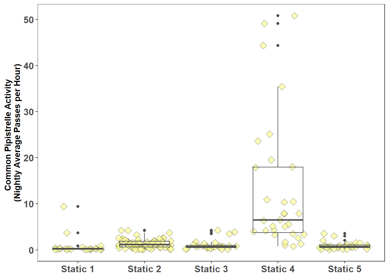
Figure 7.3 shows Common pipistrelle activity for the static locations comparison of activity can be undertaken with the Kruskal-Wallis test with the following hypothesis:
The Null Hypothesis: bat pass rates per hour are from distributions with the same median.
The Alternative Hypothesis: bat pass rates per hour are from distributions with a different median.
Show the code
# Add data and time information to the statics data using the iBats::date_time_infostatics_plus <- iBats::date_time_info(statics)# Add sun and night time metrics to the statics data using the iBats::sun_night_metrics() function.statics_plus <- iBats::sun_night_metrics(statics_plus)graph_data <- statics_plus %>%filter(Species =="Pipistrellus pipistrellus") %>%group_by(Description, Night, night_length_hr) %>%# count number of passes per night by species - makes coloumn "n""tally() %>%# calculate average bat passes per hour for each Night and speciesmutate(ave_act_per_hr = n / night_length_hr) %>%# Remove Night Length column from the Tableselect(-night_length_hr, -n) ggplot(graph_data, aes(y = ave_act_per_hr, x = Description)) +geom_jitter(fill ="#ffff99", #Common Pipistrelle colourcolour ="black", shape =23, alpha =0.7, size =3) +geom_boxplot(colour ="grey30", fill ="transparent") +labs(y ="Common Pipistrelle Activity \n(Nightly Average Passes per Hour)") +theme_bw() +theme(legend.position ="none", # No legendaxis.text.x =element_text(size=12, face="bold"), axis.text.y =element_text(size=12,face="bold"), axis.title.y =element_text(face="bold"), axis.title.x =element_blank(), # no y title (just bat names)panel.grid.major =element_blank(), #remove grid linespanel.grid.minor =element_blank())
Figure 7.3: Common Pipistrelle Activity at Each Static (Nightly Average Passes per Hour)
Show the code
# Add data and time information to the statics data using the iBats::date_time_infostatics_plus <- iBats::date_time_info(statics)# Add sun and night time metrics to the statics data using the iBats::sun_night_metrics() function.statics_plus <- iBats::sun_night_metrics(statics_plus)test_data <- statics_plus %>%filter(Species =="Pipistrellus pipistrellus") %>%group_by(Description, Night, night_length_hr) %>%# count number of passes per night by species - makes coloumn "n""tally() %>%# calculate average bat passes per hour for each Night and speciesmutate(ave_act_per_hr = n / night_length_hr) %>%# Remove Night Length column from the Tableselect(-night_length_hr, -n)# Check at least 2 locations and a minimum of 5 observations per location# Only do KW on locations with 5 or more observations# if just two locations do Mann Whitneycheck_data <- test_data %>%group_by(Description) %>%tally()# filter for Statics with more than 5 valuesStaticsWithPlus5 <- check_data %>%filter(n >=5) %>%pull(Description)test_data <- test_data %>%filter(Description %in% StaticsWithPlus5)# Extract the p-value from the kruskal.teststat_pvalue <-kruskal.test(ave_act_per_hr ~ Description, data = test_data)$p.value
The Kruskal-Wallis test undertaken for the Common pipistrelle at the following static locations: Static 1, Static 2, Static 3, Static 4, and Static 5 produced a P value (3.30e-16) less than the chosen threshold for statistical significance of 0.05; therefore the null hypothesis is rejected, activity between some static locations is likely to be different. The Dunn’s test can be applied to determine the static locations that are different.
Results of the Dunn’s test, performed after the Kruskal-Wallis test (post hoc), are shown in Table 7.4.
Show the code
df <-tibble(dunn_result$comparisons, dunn_result$P.adjusted)colnames(df) <-c("Comparison", "P.adj")resultsTable <- df %>%filter(P.adj <0.05) %>%select(`Locations with a significant difference (P<0.05)`= Comparison, `adjusted P `= P.adj)resultsTable %>%flextable(col_keys =colnames(.)) %>%fontsize(part ="header", size =12) %>%fontsize(part ="body", size =12) %>%bold(part ="header") %>%autofit(add_w =0.1, add_h =0.1) %>%bg(bg ="black", part ="header") %>%color(color ="white", part ="header") %>%align(align ="center", part ="header") %>%align(j =2, align ="right", part ="body") %>%bold(j =1, bold =TRUE, part ="body")
Table 7.4: Results of Post-hoc testing with the Dunn’s Test
Locations with a significant difference (P<0.05)
adjusted P
Static 1 - Static 2
0.0000939731690135662070
Static 1 - Static 3
0.0460478959637407314620
Static 1 - Static 4
0.0000000000000007857217
Static 2 - Static 4
0.0000001079868368327319
Static 3 - Static 4
0.0000000296352155723235
Static 4 - Static 5
0.0000000014826746844802
Table 7.4 gives the results of the post hoc testing with the Dunn’s test; post P value adjustment with the Bonferroni method showing:
Common pipistrelle activity at static 4 is significantly different (at P<0.05) to all the other static locations.
Common pipistrelle activity at static 1 is significantly different to static locations 2, 3 and 4. The significant difference (at P<0.05) between static 1 and static 3 is not easily determined from Figure 7.3.
Common pipistrelle activity at static 2, static 3, and static 5 are not significantly different (at P<0.05).
7.5 Bootstrap Confidence Intervals
Table 7.5 gives summary statistics for Barbastelle (Barbastelle barbastellus) pass observations per night at Static 5.
Show the code
# Libraries (Packages) usedlibrary(tidyverse)library(mosaic)library(gt)library(gtExtras)library(iBats)library(infer)# Add data and time information to the statics data using the iBats::date_time_infostatics_plus <- iBats::date_time_info(statics)# Group by Description and Night and Count the Observationsbarb_static5 <- statics_plus %>%filter(Species =="Barbastella barbastellus", Description =="Static 5") %>%group_by(Description, Night) %>%tally() # The summary statistics are saved into a variable riven_cond_stats cond_stats <-favstats(n~Description, data = barb_static5)# riven_cond_stats is made into a the table (using the code below)cond_stats %>%# Create the table with the gt packagegt() %>%# Style the header to black fill and white texttab_style(style =list(cell_fill(color ="black"),cell_text(color ="white", weight ="bold")),locations =cells_column_labels(columns =c(everything()) ) ) %>%#gt_color_rows(median, palette = "ggsci::yellow_material") %>% tab_options(data_row.padding =px(2))
Table 7.5: Barbastelle Observations (Passes) at Static 5
Description
min
Q1
median
Q3
max
mean
sd
n
missing
Static 5
1
1
2
4
11
3.173913
2.639769
23
0
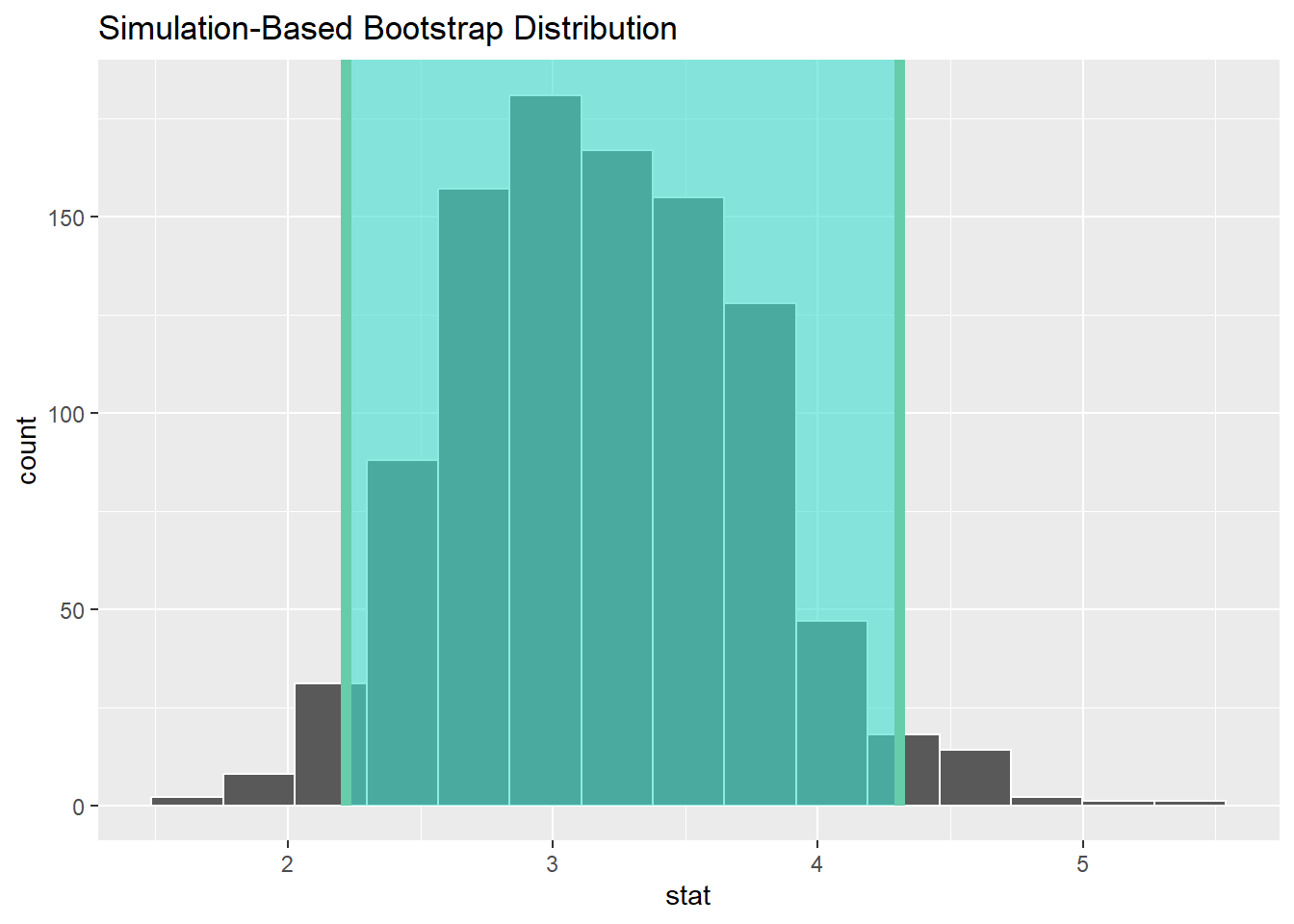
For Static 5 there is a mean of 3.17 passes per night for the 23 nights the bat detector was deployed. It is valuable to know the confidence of this mean number of passes observed. The population of passes, the number of Barbastelle’s passes for every night in history, is not available; in practice there is only the sample of data and not the entire population. The bootstrap (Glossary B.3.2) is a statistical method that allows us to approximate the sampling distribution (and therefore confidence intervals) even without access to the population.
In bootstrapping the sample itself becomes the population. Samples from the population are drawn many times over and every time from all the population. This process is called re-sampling with replacement and creates a bootstrap distribution. The infer package has functions for re-sampling with replacement and estimating confidence limits.
Show the code
# bootstrap the number of Barb pass 1000 time and calculate the mean bootstrap_distribution <- barb_static5 %>%specify(response = n) %>%generate(reps =1000, type ="bootstrap") %>%calculate(stat ="mean")#calculation the 95% confidence intervalspercentile_ci <- bootstrap_distribution %>%get_confidence_interval(level =0.95, type ="percentile")
The 95% confidence interval is computed by piping bootstrap_distribution into the get_confidence_interval() function from the infer package, with the confidence level set to 0.95 and the confidence interval type to be “percentile”. The results are saved in percentile_ci.
The 95% confidence interval is the middle 95% of values of the bootstrap distribution, the 2.5th and 97.5th percentiles, which are percentile_ci$lower_ci = 2.22 and percentile_ci$lower_ci = 4.31, respectively. This is known as the percentile method for constructing confidence intervals.
The confidence interval (2.22, 4.31) can be visualized, see Figure 7.4, by piping the bootstrap_distribution data frame into the visualize() function and adding a shade_confidence_interval() layer. The endpoints argument are set to the percentile_ci.
Figure 7.4: Boostrap Distribution of the Mean Barbastelle Observations (Passes) at Static 5
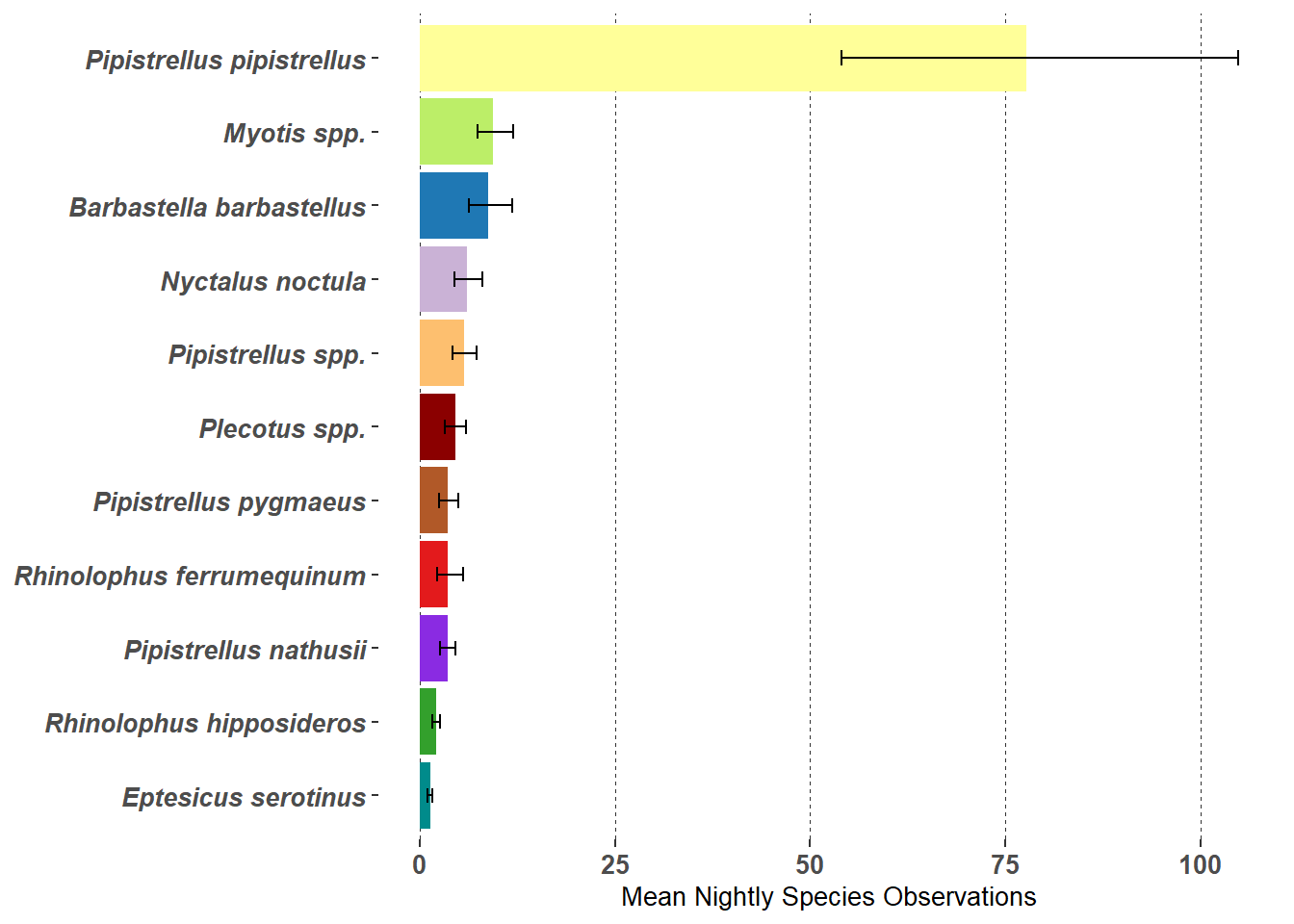
The bootstrapping of confidence intervals can be used for all the factors in a description (e.g. static locations), the month of activity or the species observed. The code below creates Table 7.6; confidence intervals for nightly species observations (passes) where there is more than 10 bat observations (passes) for the species in total. Figure 7.5 illustrates the mean nightly species observations with error bars indicating the confidence intervals.
Show the code
#List species with more than 10 passes observedSpeciesList <- statics_plus %>%group_by(Species) %>%count() %>%filter(n >10)SpeciesList <-levels(factor(SpeciesList$Species))Table_ci <-NULL#blank data.frame for tablefor(BatName in SpeciesList) { night_obs <- statics_plus %>%#filter(Species == "Pipistrellus pipistrellus", Description == static) %>% #group_by(Description, Night) %>% filter(Species == BatName) %>%group_by(Species, Night) %>%tally() # Calculate the mean species_mean <-mean(night_obs$n)# bootstrap the number of Barb pass 1000 time and calculate the mean bootstrap_distribution <- night_obs %>%specify(response = n) %>%generate(reps =1000, type ="bootstrap") %>%calculate(stat ="mean")#calculation the 95% confidence intervals species_ci <- bootstrap_distribution %>%get_confidence_interval(level =0.95, type ="percentile") species_ci$mean <- species_mean species_ci$species <- BatName Table_ci <-rbind(Table_ci, species_ci)}Table_ci %>%# round numbers to 1 decimal placemutate(mean =round(mean, digits =1),lower_ci =round(lower_ci, digits =1),upper_ci =round(upper_ci, digits =1)) %>%#Arrange descending for readabilityarrange(desc(mean)) %>%# configure column headingsselect(Species = species, Mean = mean, `Lower 95% ci`= lower_ci, `Upper 95% ci`= upper_ci) %>%gt() %>%# Style the header to black fill and white texttab_style(style =list(cell_fill(color ="black"),cell_text(color ="white", weight ="bold")),locations =cells_column_labels(columns =c(everything()) ) ) %>%# Make bat scientific name italictab_style(style =list(cell_text(style ="italic") ),locations =cells_body(columns =c(Species) ) ) %>%tab_footnote(footnote ="Species with more than 10 bat observations (passes) in total",locations =cells_column_labels(columns = Species )) %>%tab_options(data_row.padding =px(2))
Table 7.6: Nightly Species Observations (Passes) Mean and 95% Confidence Intervals
Species1
Mean
Lower 95% ci
Upper 95% ci
Pipistrellus pipistrellus
77.7
54.1
104.9
Myotis spp.
9.5
7.5
11.9
Barbastella barbastellus
8.7
6.3
11.8
Nyctalus noctula
6.1
4.4
8.1
Pipistrellus spp.
5.7
4.2
7.4
Plecotus spp.
4.5
3.2
6.0
Pipistrellus nathusii
3.6
2.6
4.6
Pipistrellus pygmaeus
3.6
2.5
4.9
Rhinolophus ferrumequinum
3.6
2.3
5.6
Rhinolophus hipposideros
2.1
1.7
2.6
Eptesicus serotinus
1.3
1.0
1.7
1 Species with more than 10 bat observations (passes) in total
Show the code
graph_bat_colours <- iBats::bat_colours_default(Table_ci$species)Table_ci %>%ggplot(aes(x=reorder(species, mean), y=mean, fill=species)) +geom_bar(position=position_dodge(), stat="identity") +geom_errorbar(aes(ymin=lower_ci, ymax=upper_ci),width=.2, # Width of the error barsposition=position_dodge(.9)) +scale_fill_manual(values = graph_bat_colours) +coord_flip() +labs(y ="Mean Nightly Species Observations") +theme_bw() +theme(legend.position ="none", # No legendaxis.text.x =element_text(size =10, angle =0, face ="bold"),axis.text.y =element_text(size =10, face ="bold.italic"), # bat names italicaxis.title.y =element_blank(), # no y title (just bat names)axis.title.x =element_text(size =10), # no x titlepanel.grid.major =element_blank(), # remove grid linespanel.grid.minor =element_blank(),panel.border =element_blank(),panel.grid.major.x =element_line(colour ="grey20", linewidth =0.1, linetype ="dashed") )
Figure 7.5: Nightly Species Observations (Passes) and 95% Confidence Intervals (error bars)
7.6 Bat Assemblage
The assessment of individual species ignores the fact there is also the species assemblage; the taxonomically related group of species (i.e. bats) occupying the same geographical area at the same time. The assemblage of bat species can be explored using multivariate methods.
For most surveys the number of species observed is greater than one, making it a biological assemblage. We can relate this assemblage to other factors such as location, habitat, time, weather, etc. Multivariate analysis gives a way of exploring the bat assemblage differences with respect to factors such as the location/habitat or month/year or combination of both.
7.6.1 Cluster Analysis
Table 7.7 shows a summary matrix of bat passes per species for each static (i.e. location) We would like to know which locations are similar/dissimilar.
In multivariate analysis the pre-treament of data (sometimes in more than one way) is usually desirable (Glossary B.7.1). For assemblage data, transformations will reduce the dominant contribution of abundant species (i.e. all those pips). Transformations include (None, Square root, Fourth root, Log(X+1), Presence/absence). Table 7.8 shows Table 7.7 transformed with the species \(\sqrt[2]{count}\).
Show the code
SpeciesC <- Tab_L_S %>%ungroup() %>%select(2:ncol(.)) %>%mutate_all(funs(sqrt(.)))Table <- SpeciesC %>%mutate_all(funs(round(., 2)))Matrix <- Tab_L_S %>%ungroup() %>%select(Description) %>%bind_cols(SpeciesC)MatrixTable <- Tab_L_S %>%ungroup() %>%select(Description) %>%bind_cols(Table)Matrix <-data.matrix(Matrix[, 2:ncol(Matrix)])r_names <- Tab_L_S %>%ungroup() %>%pull(Description)rownames(Matrix) <- r_names# Number of columns in tablencols <-ncol(MatrixTable)#Make coloured palettecolourer <- scales::col_numeric(palette =c("transparent", "forestgreen"),domain =c(0, maxValue))MatrixTable %>%flextable() %>%bold(part ="header") %>%bg(bg ="black", part ="header") %>%color(color ="white", part ="header") %>%rotate(j =2:ncols, rotation ="tbrl", align ="center", part ="header") %>%height_all(height =2.3, part ="header") %>%hrule(rule ="exact", part ="header") %>%bg(bg = colourer, j =2:ncols, part ="body") %>%width(j =2:ncols, width =0.4) %>%width(j =1, width =0.8)
Table 7.8: Transformed Matrix
Description
Barbastella barbastellus
Eptesicus serotinus
Myotis nattereri
Myotis spp.
Nyctalus leisleri
Nyctalus noctula
Nyctalus spp.
Pipistrellus nathusii
Pipistrellus pipistrellus
Pipistrellus pygmaeus
Pipistrellus spp.
Plecotus spp.
Rhinolophus ferrumequinum
Rhinolophus hipposideros
Static 1
2.00
0.00
0
8.19
0.00
5.92
0.00
1.41
12.12
1.73
2.00
0.00
0.00
0.00
Static 2
5.29
2.00
1
12.96
0.00
14.18
0.00
3.16
27.53
4.69
6.00
9.75
7.75
5.29
Static 3
3.16
0.00
1
6.40
1.73
5.92
0.00
4.24
16.22
3.87
4.36
4.47
9.00
6.00
Static 4
17.44
2.83
0
9.22
0.00
5.29
0.00
1.41
59.74
6.24
11.66
4.47
3.74
2.83
Static 5
8.54
0.00
0
8.60
0.00
4.00
1.41
0.00
15.33
2.65
9.38
1.00
2.24
1.00
To assess the differences of activity (in the bat assemblage) between locations (or months, habitat, etc.) we measure the distance between every point of activity with every other point. So activity (e.g. a median or count) at one location for a species is compared(measured) with every other activity for all the species and locations.
There are many distance measurements to investigate species similarity/dissimilarity3 for more information see the Glossary B.7.5
In this example the Bray-Curtis distance measurement (Glossary B.7.10) has been applied to Table 7.8 to produce the Bray-Curtis dissimilarity matrix in Table 7.9.
(For species similarities it may be worth considering the removal of the rarer species (i.e. the less observed) and repeating the analysis.)
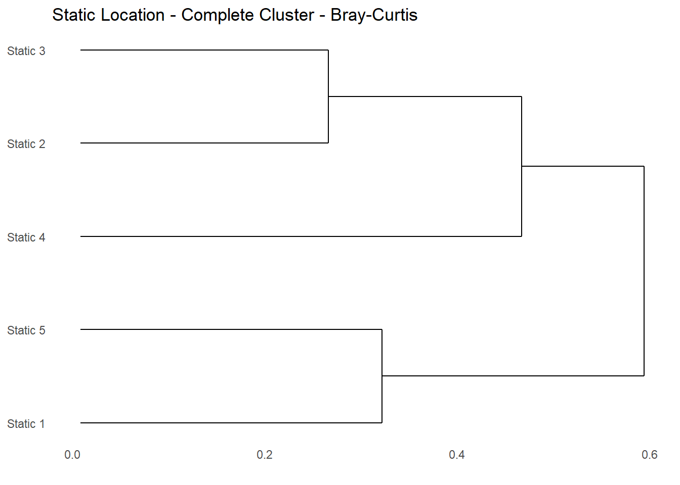
The Bray-Curtis dissimilarity matrix can be used in many multivariate methods; here the matix is used in Hierarchical Clustering (Glossary B.7.13). Hierarchical clustering is useful because it can create a tree-based representation of the observations called a dendrogram (Glossary B.7.15); that is easy to interpret visually. The dendrogram from the Bray-Curtis dissimilarity matrix in Table 7.9 is shown in Figure 7.6.
Clustering refers to a very broad set of techniques for finding subgroups, or clusters, in a data set. Clustering involves grouping a set of objects in such a way that objects in the same group (called a cluster) are more similar (in some sense) to each other than to those in other groups (clusters). Referring to the dendrogram in Figure 7.6 the lower in the tree fusions occur, the more similar the groups of observations are to each other. While observations that fuse later, near the top of the tree, can be considered less similar.
For Figure 7.6 we can see that for the bat assemblage:
Statics 3 & 2 are similar
Statics 1 & 5 are similar
Static 4 is more similar to Statics 2 & 3 than Statics 1 & 5
Statics 2 & 3 and Statics 1 & 5 are more similar to Static 4 - than Statics 2 & 3 and Statics 1 & 5 are to each other
Note, the dendrogram is illustrative and we cannot draw conclusions about the degree of similarity of two observations based on their proximity along the vertical axis.
This is just an introduction to Hierarchical Clustering, there are many variations and other types of clustering (e.g. k-means). Key variations for hierarchical clustering are:
distance measurement used e.g. Bray-Curtis, Euclidean, etc.
type of linkage e.g. complete, average, single or centroid.
7.6.2 K-Means Clustering
K-means clustering (Glossary B.7.17) is a simple approach for partitioning a data set into K distinct non-overlapping clusters. To perform K means clustering we must specify the desired number of clusters first. The code below applies k-means clustering to the Bray-Curtis dissimilarity matrix in Table 7.9 with K=2.
withinss: Table 7.11 Vector of within-cluster sum of squares, one component per cluster.
tot.withinss: Table 7.12 Total within-cluster sum of squares, i.e. sum(withinss).
betweenss: Table 7.12 The between-cluster sum of squares, i.e. \(totss-tot.withinss\).
size: The number of points in each cluster.
iter: Table 7.12 The number of (outer) iterations.
7.6.3 Non-metric Multidimensional Scaling (NMDS)
Non-metric Multidimensional Scaling (Glossary B.7.20) is an ordination technique that reduces dimensionality in multivariate data sets such as the count of bats in Table 7.13. Dimensionality reduction simply refers to the process of reducing the number of attributes in a dataset while keeping as much of the variation in the original dataset as possible. The goal of NMDS is to collapse information from multiple dimensions (e.g, from multiple communities, sites, etc.) into just a few, so that they can be visualized, (e.g. as a 2D or 3D plot), and interpreted.
Unlike other ordination techniques that rely on (primarily Euclidean) distances, such as Principal Component Analysis (PCA), NMDS uses rank orders, and thus is an extremely flexible technique that can accommodate a variety of different kinds of data (K. R. Clarke 1993), (K. Robert Clarke 1999); NMDS does require at least one observation per factor (e.g. site or month). In R, the metaMDS() function of the vegan package can execute a NMDS. As input, it expects a community matrix with the factors as rows and the species as columns; Table 7.13 has two factors, static location and month, that are treated separately.
Before undertaking ordination it is best to transform the data; this helps reduce the influence of large counts from dominant species (i.e. Common pipistrelles). Table 7.14 is Table 7.13 transformed with \(\sqrt[4]{count}\).
A measure of how successful the NMDS reduction is stress4. The lower the stress value, the better the ordination. A rule of thumb for stress values:
stress < 0.05 provides an excellent representation in reduced dimensions
stress < 0.1 is great,
stress < 0.2 is good,
stress > 2.0 < 0.3 interpret with caution
stress > 0.3 provides a poor representation.
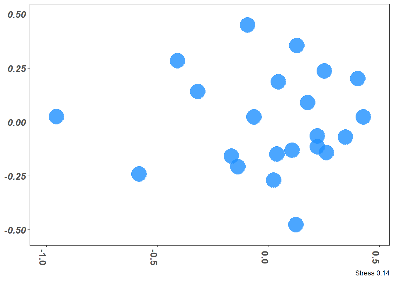
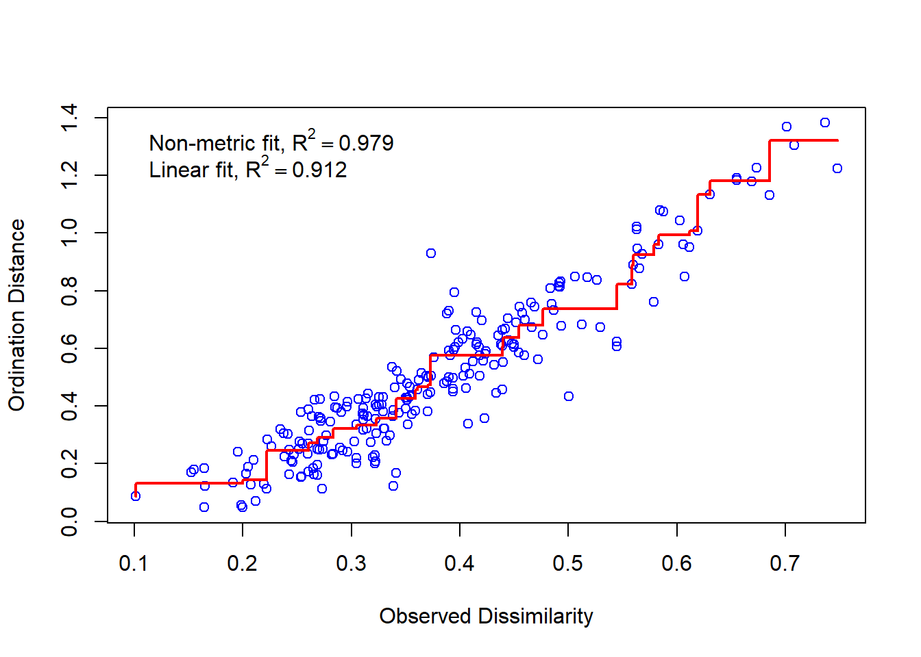
Figure 7.7 (a) shows the two dimensional plot after the NMDS is applied through metaMDS() function to the transformed data shown in Table 7.14; the NMDS produced a good stress of 0.14. Figure 7.7 (b) is the Shepard plot (Glossary B.7.20.1) showing the scatter around the regression between the interpoint distances in the final configuration (i.e., the distances between each pair of communities) against their original dissimilarities; the desirable outcome from the Shepard plot is a diagonal line with limited scatter in this respect Figure 7.7 (b) looks reasonable.
library(tidyverse)library(glue)library(ggthemes) # for colour pallet "Tableau 10"
Attaching package: 'ggthemes'
The following object is masked from 'package:mosaic':

    theme_map
Show the code
library(flextable)library(iBats)library(vegan)# Add data and time information to the statics data using the iBats::date_time_infostatics_plus <- iBats::date_time_info(statics)# Count of bat species by location and monthdescription_month_count <- statics_plus %>%# Location - Speciesgroup_by(Species, Description, Month) %>%count() %>%pivot_wider(names_from = Species, values_from = n) %>%replace(is.na(.), 0)# Number of columns in tablencols <-ncol(description_month_count)description_month_count %>%flextable() %>%bold(part ="header") %>%bg(bg ="black", part ="header") %>%color(color ="white", part ="header") %>%rotate(j =3:ncols, rotation ="tbrl", align ="center", part ="header") %>%height_all(height =2.3, part ="header") %>%hrule(rule ="exact", part ="header") %>%width(j =3:ncols, width =0.4) %>%width(j =1:2, width =0.8)
Table 7.13: Count of Species by the Meta Data; Location and month
Description
Month
Barbastella barbastellus
Eptesicus serotinus
Myotis nattereri
Myotis spp.
Nyctalus leisleri
Nyctalus noctula
Nyctalus spp.
Pipistrellus nathusii
Pipistrellus pipistrellus
Pipistrellus pygmaeus
Pipistrellus spp.
Plecotus spp.
Rhinolophus ferrumequinum
Rhinolophus hipposideros
Static 1
Aug
4
0
0
58
0
12
0
0
20
0
1
0
0
0
Static 2
May
7
1
0
1
0
4
0
2
128
0
6
2
2
2
Static 2
Jun
6
2
1
3
0
32
0
0
163
0
5
0
23
6
Static 2
Aug
10
1
0
103
0
137
0
0
260
17
6
14
18
4
Static 2
Sep
3
0
0
35
0
4
0
8
108
5
16
32
9
7
Static 2
Oct
2
0
0
9
0
2
0
0
20
0
2
47
1
7
Static 3
Jun
2
0
1
2
0
8
0
0
33
0
1
0
13
3
Static 3
Aug
2
0
0
22
3
19
0
0
153
5
5
6
6
15
Static 3
Sep
6
0
0
17
0
6
0
17
40
9
10
13
55
10
Static 4
Jun
161
0
0
9
0
7
0
0
379
1
9
0
7
2
Static 4
Jul
22
2
0
20
0
1
0
0
1,644
6
48
1
0
1
Static 4
Aug
83
6
0
37
0
20
0
0
1,318
29
48
19
6
4
Static 4
Oct
38
0
0
19
0
0
0
2
228
3
31
0
1
1
Static 5
Jun
29
0
0
2
0
12
2
0
66
0
9
1
4
0
Static 5
Jul
27
0
0
25
0
0
0
0
65
1
22
0
0
1
Static 5
Aug
10
0
0
37
0
4
0
0
72
6
42
0
1
0
Static 5
Oct
7
0
0
10
0
0
0
0
32
0
15
0
0
0
Static 1
May
0
0
0
1
0
4
0
0
4
0
0
0
0
0
Static 1
Sep
0
0
0
8
0
3
0
2
11
3
2
0
0
0
Static 2
Jul
0
0
0
17
0
22
0
0
79
0
1
0
7
2
Static 1
Jun
0
0
0
0
0
16
0
0
112
0
1
0
0
0
Static 3
May
0
0
0
0
0
2
0
1
37
1
3
1
7
8
Show the code
species_count <- description_month_count[, 3:ncol(description_month_count)]meta_data <- description_month_count[, 1:2]Transformed_Data <- (species_count)^(1/4)# Number of columns in tablencols <-ncol(Transformed_Data)Transformed_Data %>%flextable() %>%bold(part ="header") %>%bg(bg ="black", part ="header") %>%color(color ="white", part ="header") %>%rotate(j =1:ncols, rotation ="tbrl", align ="center", part ="header") %>%height_all(height =2.3, part ="header") %>%hrule(rule ="exact", part ="header") %>%width(j =1:ncols, width =0.4) %>%colformat_double(digits =3)
Table 7.14: Count of Species with Data Transformed by 4th Root
Barbastella barbastellus
Eptesicus serotinus
Myotis nattereri
Myotis spp.
Nyctalus leisleri
Nyctalus noctula
Nyctalus spp.
Pipistrellus nathusii
Pipistrellus pipistrellus
Pipistrellus pygmaeus
Pipistrellus spp.
Plecotus spp.
Rhinolophus ferrumequinum
Rhinolophus hipposideros
1.414
0.000
0.000
2.760
0.000
1.861
0.000
0.000
2.115
0.000
1.000
0.000
0.000
0.000
1.627
1.000
0.000
1.000
0.000
1.414
0.000
1.189
3.364
0.000
1.565
1.189
1.189
1.189
1.565
1.189
1.000
1.316
0.000
2.378
0.000
0.000
3.573
0.000
1.495
0.000
2.190
1.565
1.778
1.000
0.000
3.186
0.000
3.421
0.000
0.000
4.016
2.031
1.565
1.934
2.060
1.414
1.316
0.000
0.000
2.432
0.000
1.414
0.000
1.682
3.224
1.495
2.000
2.378
1.732
1.627
1.189
0.000
0.000
1.732
0.000
1.189
0.000
0.000
2.115
0.000
1.189
2.618
1.000
1.627
1.189
0.000
1.000
1.189
0.000
1.682
0.000
0.000
2.397
0.000
1.000
0.000
1.899
1.316
1.189
0.000
0.000
2.166
1.316
2.088
0.000
0.000
3.517
1.495
1.495
1.565
1.565
1.968
1.565
0.000
0.000
2.031
0.000
1.565
0.000
2.031
2.515
1.732
1.778
1.899
2.723
1.778
3.562
0.000
0.000
1.732
0.000
1.627
0.000
0.000
4.412
1.000
1.732
0.000
1.627
1.189
2.166
1.189
0.000
2.115
0.000
1.000
0.000
0.000
6.368
1.565
2.632
1.000
0.000
1.000
3.018
1.565
0.000
2.466
0.000
2.115
0.000
0.000
6.025
2.321
2.632
2.088
1.565
1.414
2.483
0.000
0.000
2.088
0.000
0.000
0.000
1.189
3.886
1.316
2.360
0.000
1.000
1.000
2.321
0.000
0.000
1.189
0.000
1.861
1.189
0.000
2.850
0.000
1.732
1.000
1.414
0.000
2.280
0.000
0.000
2.236
0.000
0.000
0.000
0.000
2.839
1.000
2.166
0.000
0.000
1.000
1.778
0.000
0.000
2.466
0.000
1.414
0.000
0.000
2.913
1.565
2.546
0.000
1.000
0.000
1.627
0.000
0.000
1.778
0.000
0.000
0.000
0.000
2.378
0.000
1.968
0.000
0.000
0.000
0.000
0.000
0.000
1.000
0.000
1.414
0.000
0.000
1.414
0.000
0.000
0.000
0.000
0.000
0.000
0.000
0.000
1.682
0.000
1.316
0.000
1.189
1.821
1.316
1.189
0.000
0.000
0.000
0.000
0.000
0.000
2.031
0.000
2.166
0.000
0.000
2.981
0.000
1.000
0.000
1.627
1.189
0.000
0.000
0.000
0.000
0.000
2.000
0.000
0.000
3.253
0.000
1.000
0.000
0.000
0.000
0.000
0.000
0.000
0.000
0.000
1.189
0.000
1.000
2.466
1.000
1.316
1.000
1.627
1.682
Show the code
# Nonmetric Multidimensional Scaling (NMDS), # and tries to find a stable solution # using several random startsnMDS_results <-metaMDS(Transformed_Data, distance ="bray")# extract NMDS scores (x and y coordinates) for plottingnMDS_coords =as_tibble(scores(nMDS_results)$sites)# bind the factors (static location and month back)graph_data <-bind_cols(meta_data, nMDS_coords)
Show the code
graph_style <-theme_bw() +theme(legend.position ="none", # No legendaxis.text.x =element_text(size=12, angle =270, face="bold"), # text bold and verticalaxis.text.y =element_text(size=12, face="bold.italic"), # bat names italicstrip.text =element_text(size=12, face="bold"), # Bold facet namesaxis.title.x =element_blank(), # currently not usedaxis.title.y =element_blank(), # no y title (just bat names)panel.grid.major =element_blank(), #remove grid linespanel.grid.minor =element_blank(),plot.caption =element_text())g1 <-ggplot(graph_data, aes(x = NMDS1, y = NMDS2)) +geom_point(size =9, colour ="dodgerblue", alpha =0.8) +scale_x_continuous(expand =c(0.05, 0.05)) +scale_y_continuous(expand =c(0.05, 0.05)) +labs(caption =glue("Stress {round(nMDS_results$stress, digits = 2)}")) + graph_styleg1stressplot(nMDS_results)
(a) Unlabeled Solution of NMDS (2D)
(b) Stress Plot
Figure 7.7: Non-metric Multidimensional Scaling Solution and Stress Plot
Figure 7.8: Non-metric Multidimensional Scaling Solution and Stress Plot
7.6.3.1 ANOSIM
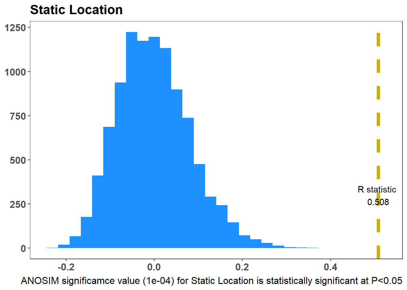
The ANOSIM test (Glossary B.7.21) is similar to an ANOVA hypothesis test; it uses a dissimilarity matrix as input instead of raw data. It is also non-parametric, meaning it doesn’t assume much about the data, a useful attribute for the often-skewed ecological data. As a non-parametric test, ANOSIM uses ranked dissimilarities instead of actual distances, and for this reason complements an NMDS plot. The main point of the ANOSIM test is to determine if the differences between two or more groups are significant.
The function anosim from the package vegan(Glossary B.8.6) can test whether there is a statistical difference between groups (e.g. static locations or months)
null hypothesis - no differnce
alternative - difference
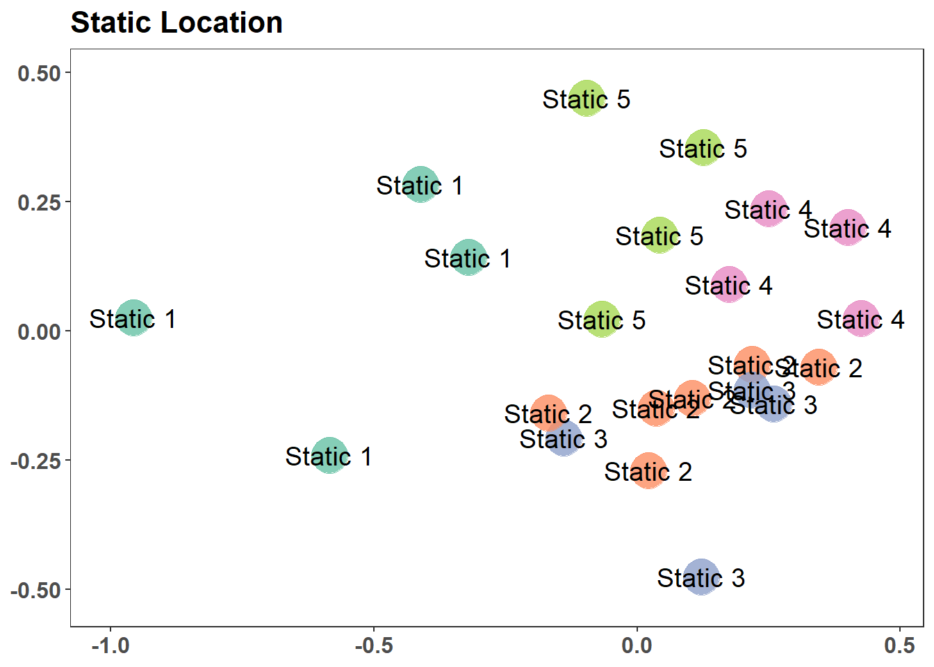
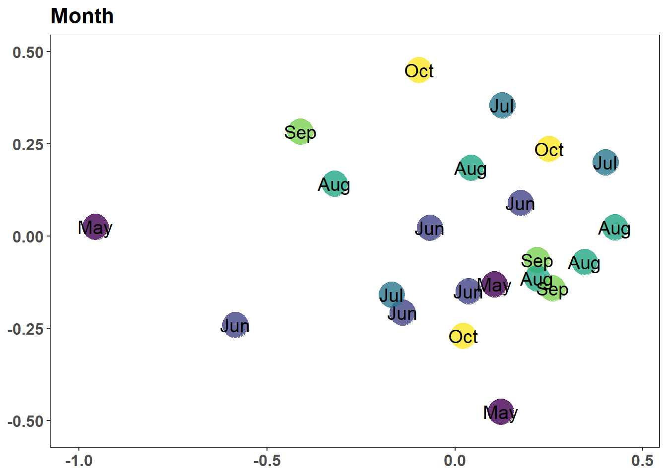
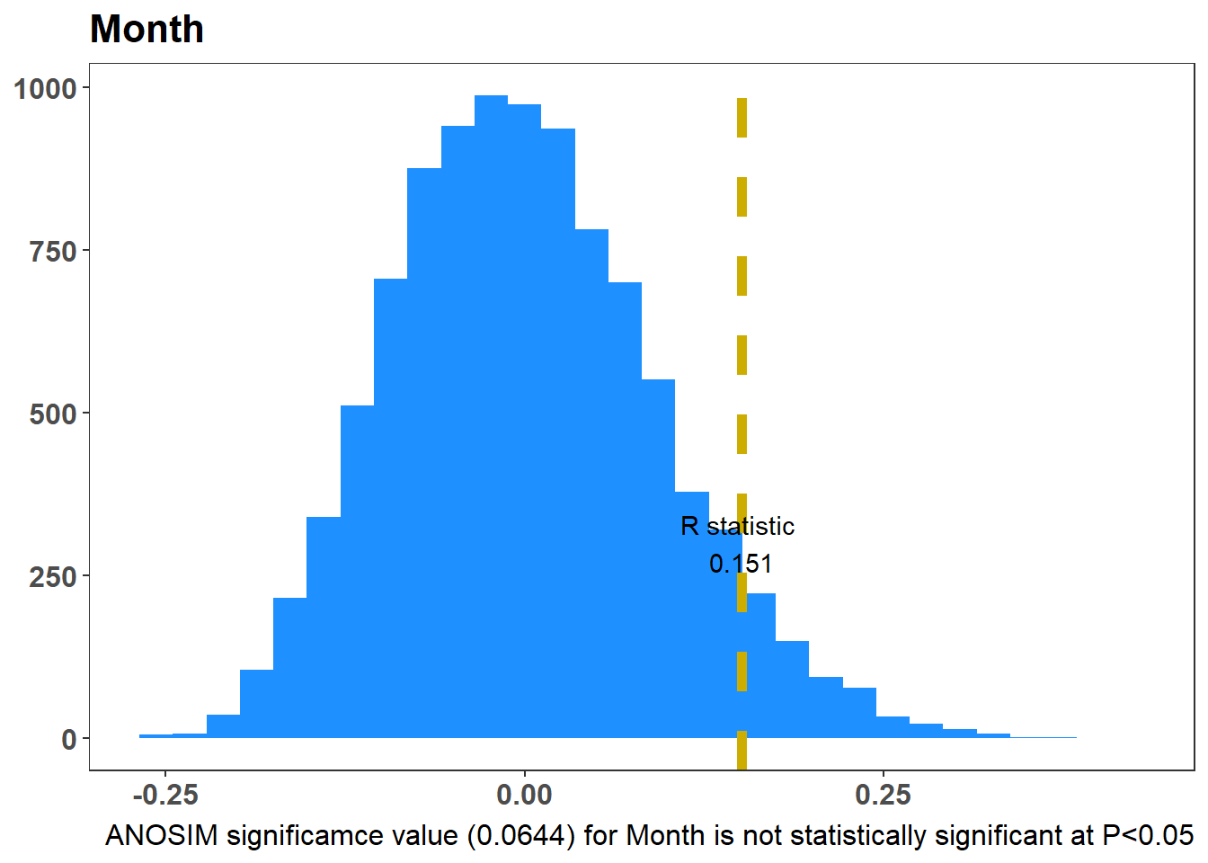
The higher the R value (it has a range 0 to 1), the more dissimilar your groups5 are in terms of bat assemblage. Figure 7.9 (a) shows the ANOSIM result for the Static Locations, there is a statistical difference of the bat species assemblage for the static location. Figure 7.9 (b) shows the ANOSIM result for the Month, there is no statistical difference of the bat species assemblage for the Months.
Show the code
graph_style <-theme_bw() +theme(legend.position ="none", axis.text.x =element_text(size=12, face="bold"),axis.text.y =element_text(size=12, face="bold"), strip.text =element_text(size=12, face="bold"), axis.title.x =element_blank(), axis.title.y =element_blank(), panel.grid.major =element_blank(), panel.grid.minor =element_blank(),plot.caption =element_text(size =12),plot.title =element_text(size=16, face="bold"))Factor <-"Static Location"ano =anosim(Transformed_Data, meta_data$Description, distance ="bray", permutations =9999)#Tjis is how PrimerE views ANOSIM ResultsRperms<-tibble(ano$perm)Rstat <- ano$statisticsigValue <- ano$signifif(sigValue <0.05) { SigText <-glue("ANOSIM significamce value ({sigValue}) for {Factor} is statistically significant at P<0.05")} else { SigText <-glue("ANOSIM significamce value ({sigValue}) for {Factor} is not statistically significant at P<0.05")}colnames(Rperms) <-c("Rano")p1_description <-ggplot(Rperms, aes(Rano)) +geom_histogram(fill ="dodgerblue") +geom_vline(xintercept = Rstat, colour ="gold3", linewidth =2, linetype ="dashed") +annotate("text", x = Rstat, y =300, label =glue("R statistic \n {round(Rstat, digits = 3)}")) +labs(title = Factor,y ="Frequency",x ="R",caption = SigText) + graph_styleFactor <-"Month"ano =anosim(Transformed_Data, meta_data$Month, distance ="bray", permutations =9999)#Tjis is how PrimerE views ANOSIM ResultsRperms<-tibble(ano$perm)Rstat <- ano$statisticsigValue <- ano$signifif(sigValue <0.05) { SigText <-glue("ANOSIM significamce value ({sigValue}) for {Factor} is statistically significant at P<0.05")} else { SigText <-glue("ANOSIM significamce value ({sigValue}) for {Factor} is not statistically significant at P<0.05")}colnames(Rperms) <-c("Rano")p2_month <-ggplot(Rperms, aes(Rano)) +geom_histogram(fill ="dodgerblue") +geom_vline(xintercept = Rstat, colour ="gold3", linewidth =2, linetype ="dashed") +annotate("text", x = Rstat, y =300, label =glue("R statistic \n {round(Rstat, digits = 3)}")) +labs(title = Factor,y ="Frequency",x ="R",caption = SigText) + graph_stylep1_descriptionp2_month
(a) ANOSIM Static Location
(b) ANOSIM Month
Figure 7.9: ANOSIM: Test is there a Statistical Difference Between Groups
7.6.4 Diversity Indices
The diversity indexes (Glossary B.7.23) are a set of metrics that quantify the diversity of a community (Magurran 2004). The most common diversity indexes are the Shannon index Shannon and Weaver (1949), the Simpson index (Simpson 1949), and the Pielou index (Simpson 1949). The Shannon index is a measure of the uncertainty in predicting the species identity of an individual chosen at random from the community. The Simpson index is a measure of the probability that two individuals randomly selected from the community will belong to the same species. The Pielou index is a measure of the evenness of the species distribution in the community. These indices go beyond simply counting the number of species (species richness) and consider how evenly distributed those species are.
It is normal for no transformation (pre-treatment) to be applied to the abundance data before calculating. However, in some cases, a log transformation (e.g. ln(x+1)) on the abundance data, could be undertaken. This can downweight the influence of highly abundant species and give more weight to rare ones, offering a more even weighting across species.
Diversity can be measured through the number of bat passes recorded on ultrasonic bat detectors, but they do introduce certain biases that can affect data interpretation. Understanding these biases is crucial for accurate data analysis and interpretation.
Bats vary their echolocation calls based on factors like prey type, hunting strategy, and social interactions.
Multiple bat species can share similar call characteristics, making it difficult to distinguish between them based on echolocation calls alone.
Different bat species use different frequency ranges for echolocation, lower frequency calls travel further than higher frequency.
Background noise from wind, rain, traffic, and other sources can interfere with call detection, especially for faint or distant calls.
7.6.4.1 Shannon Diversity Index
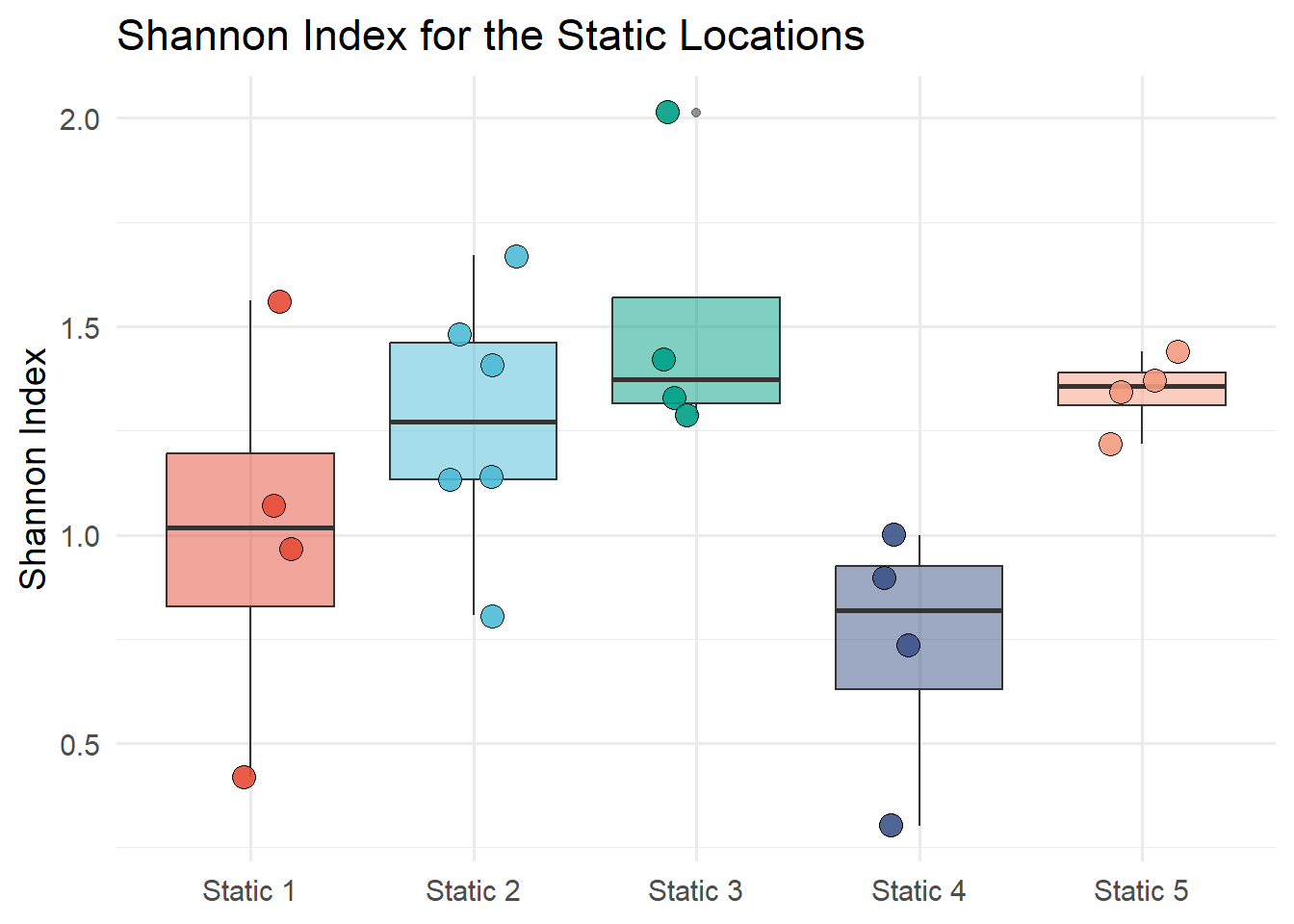
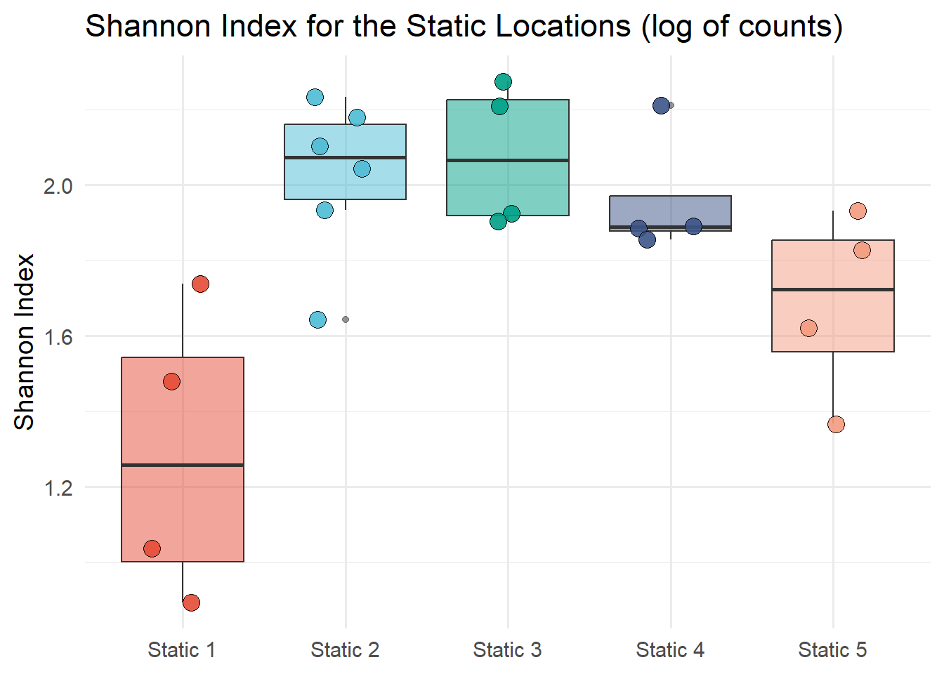
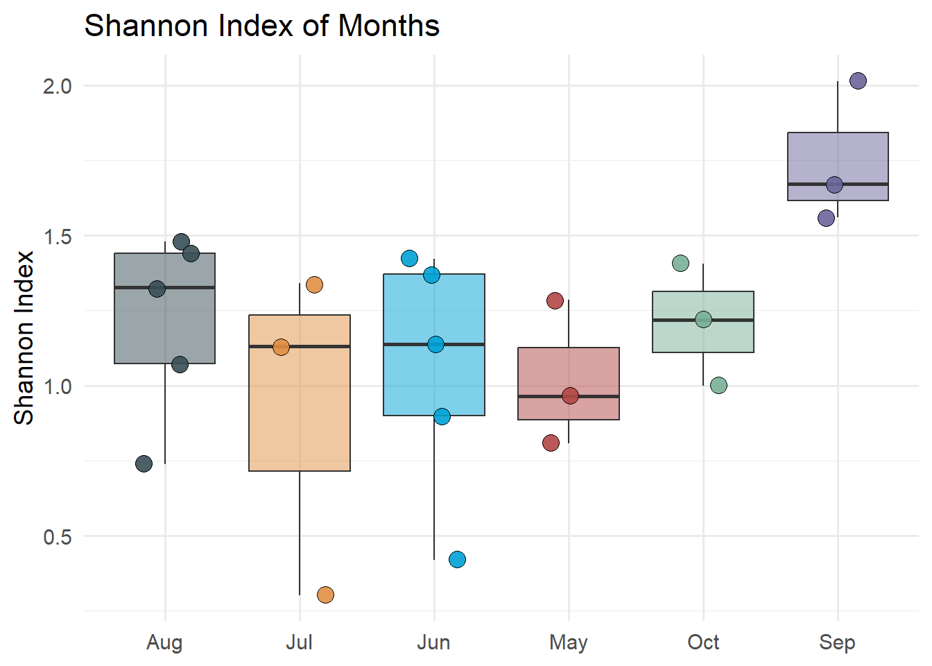
Figure 7.10 shows the Shannon diversity index of static locations. The Shannon index is calculated with the diversity function from the vegan package. The Shannon index is calculated for each static location and month and the results are plotted on a box plot by the static location. Figure 7.11 shows the Shannon diversity index of static locations with a log of counts and Figure 7.12 shows the Shannon diversity index of months.
Show the code
statics_with_night <- iBats::date_time_info(statics)static_count <- statics_with_night |>group_by(Species, Description, Month) |>summarise(n =n()) |>#Merge the Description and Month columnsunite("Description", c("Description", "Month"), sep ="_") |>pivot_wider(names_from ="Species", values_from ="n", values_fill =0) |>#make first column the description (row names)column_to_rownames(var ="Description") #Divesity index of static locationsSh <-diversity(static_count, index ="shannon")#class(Sh)# unname the Sh vectorIndex_Sh <-unname(Sh)# extract the row names from ShNames_Sh <-names(Sh)Sh_data <-tibble(Names_Sh, Index_Sh) |>separate(Names_Sh, c("Description", "Month"), sep ="_") ggplot(Sh_data, aes(x = Description, y = Index_Sh, fill = Description))+geom_boxplot(alpha =0.5) +geom_jitter(width =0.2, alpha =0.9, shape =21, size =4) +labs(title ="Shannon Index for the Static Locations",x ="Location",y ="Shannon Index") +scale_fill_npg() +theme_minimal(base_size =14) +theme(legend.position ="none",axis.title.x =element_blank())
Figure 7.10: Shannon diversity index of static locations
Show the code
# Log values of countsstatic_count_log <- static_count |>mutate(across(everything(), ~log(. +1))) #Divesity index of static locationsSh_log <-diversity(static_count_log, index ="shannon")#class(Sh)# unname the Sh vectorIndex_Sh_log <-unname(Sh_log)# extract the row names from ShNames_Sh_log <-names(Sh_log)Sh_data_log <-tibble(Names_Sh_log, Index_Sh_log) |>separate(Names_Sh_log, c("Description", "Month"), sep ="_") ggplot(Sh_data_log, aes(x = Description, y = Index_Sh_log, fill = Description))+geom_boxplot(alpha =0.5) +geom_jitter(width =0.2, alpha =0.9, shape =21, size =4) +labs(title ="Shannon Index for the Static Locations (log of counts)",x ="Location",y ="Shannon Index") +scale_fill_npg() +theme_minimal(base_size =14) +theme(legend.position ="none",axis.title.x =element_blank())
Figure 7.11: Shannon diversity index of static locations (Log of counts)
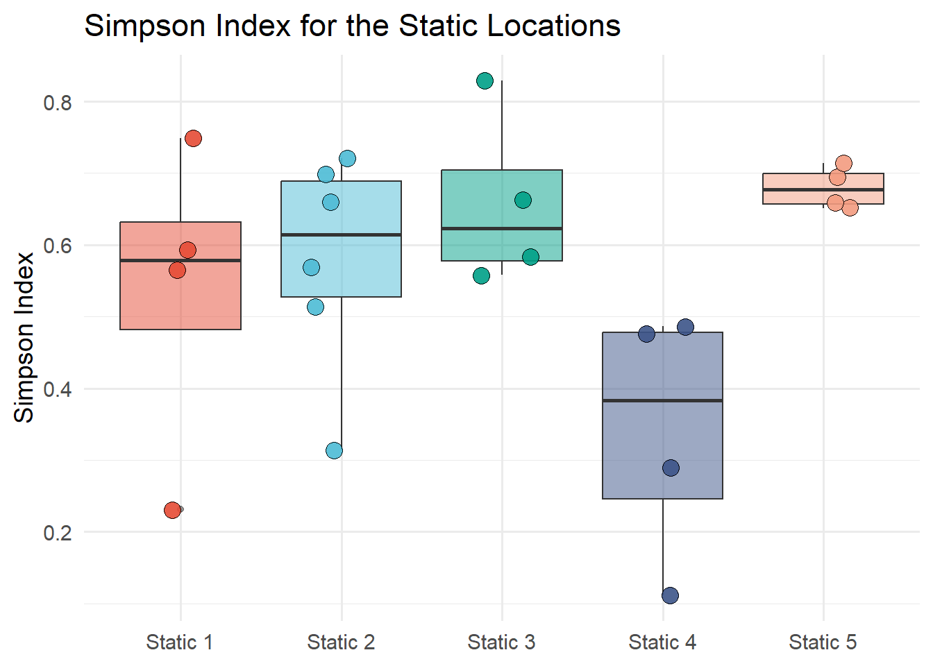
Figure 7.13 shows the Simpson diversity index of static locations. The Simpson index is calculated with the diversity function from the vegan package. The Simpson index is calculated for each static location and month and the results are plotted on a box plot by the static location.
Show the code
#Divesity index of static locationsSi <-diversity(static_count, index ="simpson")#class(Sh)# unname the Sh vectorIndex_Si <-unname(Si)# extract the row names from ShNames_Si <-names(Si)Si_data <-tibble(Names_Si, Index_Si) |>separate(Names_Si, c("Description", "Month"), sep ="_") ggplot(Sh_data, aes(x = Description, y = Index_Si, fill = Description))+geom_boxplot(alpha =0.5) +geom_jitter(width =0.2, alpha =0.9, shape =21, size =4) +labs(title ="Simpson Index for the Static Locations",x ="Location",y ="Simpson Index") +scale_fill_npg() +theme_minimal(base_size =14) +theme(legend.position ="none",axis.title.x =element_blank())
Figure 7.13: Simpson diversity index of static locations
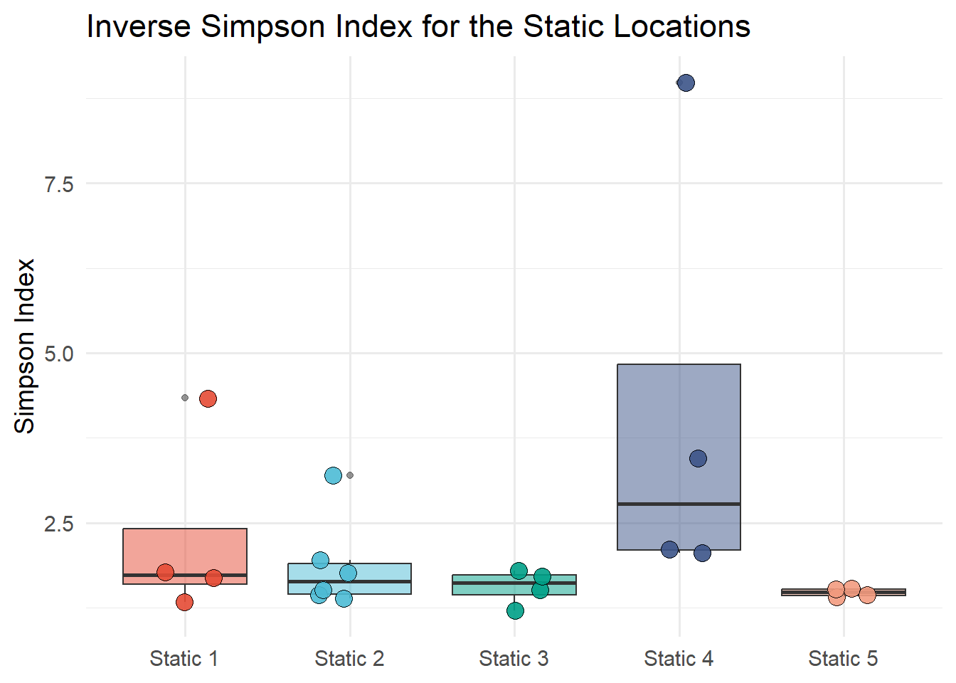
7.6.4.3 Inverse Simpson Diversity Index
Figure 7.14 shows the Inverse Simpson diversity index (\(1/D\)) of static locations. The Simpson index is calculated with the diversity function from the vegan package. The Simpson index is calculated for each static location and month and the results are plotted on a box plot by the static location.
Show the code
#Divesity index of static locationsSi <-diversity(static_count, index ="simpson")Si <-1/Si# unname the Sh vectorIndex_Si <-unname(Si)# extract the row names from ShNames_Si <-names(Si)Si_data <-tibble(Names_Si, Index_Si) |>separate(Names_Si, c("Description", "Month"), sep ="_") ggplot(Sh_data, aes(x = Description, y = Index_Si, fill = Description))+geom_boxplot(alpha =0.5) +geom_jitter(width =0.2, alpha =0.9, shape =21, size =4) +labs(title ="Inverse Simpson Index for the Static Locations",x ="Location",y ="Simpson Index") +scale_fill_npg() +theme_minimal(base_size =14) +theme(legend.position ="none",axis.title.x =element_blank())
Figure 7.14: Inverse Simpson diversity index of static locations
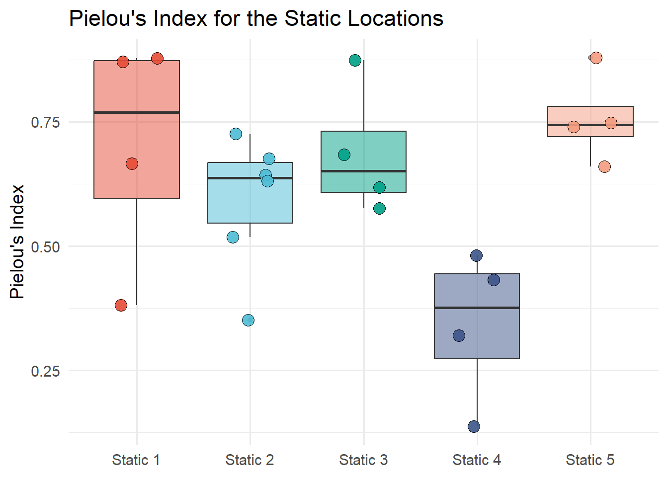
7.6.4.4 Pielou Diversity Index
The Pielou index is calculated by the equation:
\[J = \frac{H}{\ln S}\] where \(H\) is the Shannon index and \(S\) is the total number of species in the community.
The Shannon index is calculated with the diversity function from the vegan package. The total number of species can be calculated with the specnumber function from the vegan package. Figure 7.15 shows the Pielou diversity index of static locations.
Show the code
Sh <-diversity(static_count, index ="shannon")Spec_number <-specnumber(static_count)J <- Sh/log(Spec_number)#class(Sh)# unname the Sh vectorIndex_J <-unname(J)# extract the row names from ShNames_J <-names(J)J_data <-tibble(Names_J, Index_J) |>separate(Names_J, c("Description", "Month"), sep ="_")ggplot(J_data, aes(x = Description, y = Index_J, fill = Description))+geom_boxplot(alpha =0.5) +geom_jitter(width =0.2, alpha =0.9, shape =21, size =4) +labs(title ="Pielou's Index for the Static Locations",x ="Location",y ="Pielou's Index") +scale_fill_npg() +theme_minimal(base_size =14) +theme(legend.position ="none",axis.title.x =element_blank())
Figure 7.15: Pielou’s diversity index of static locations
Borcard, Daniel, Francois Gillet, and Pierre Legendre. 2011. Numerical Ecology with R. Use R! Springer Science + Business Media.
Clarke, K Robert. 1999. “Nonmetric Mutivariate Analysis in Community-Level Ecotoxicology.”Environmental Toxicology and Chemistry 18 (2): 118–27.
Clarke, K. R. 1993. “Non-Parametric Multivariate Analysis of Changes in Community Structure.”Australian Journal of Ecology 18: 117–43.
Dytham, Calvin. 2011. Choosing and UsingStatistics: ABiologist’s Guide. Third. Wiley-Blackwell.
Emden, Helmut van. 2008. Statistics for TerrifiedBiologists. Blackwell Publishing.
Fowler, Jim, Lou Cohen, and Phil Jarvis. 1998. Practical Statistics for FieldBiology. Second. Wiley.
Fox, Gordon A, Simoneta Negrete-Yankelevich, and And. 2015. Ecological Statistics. Oxford University Press. ww.oup.com.
Legendre, Pierre, and Louis Legendre. 2012. Numerical Ecology. Third English. Developments in EnvironmentalModelling. Elsevier.
Magurran, A. E. 2004. Measuring Biological Diversity. Wiley-Blackwell.
Shannon, C. E. 1948. “A Mathematical Theory of Communication.”Bell System Technical Journal 27 (3): 379–423.
Shannon, C. E., and W. Weaver. 1949. The Mathematical Theory of Communication. University of Illinois Press.
Simpson, E. H. 1949. “Measurement of Diversity.”Nature 163 (4148): 688.
Zuur, Alain F., Elena N. Ieno, and Chris S. Elphick. 2010. “A Protocol for Data Exploration to Avoid Common Statistical Problems.”Methods in Ecology and Evolution 1 (1): 3–14. https://doi.org/https://doi.org/10.1111/j.2041-210X.2009.00001.x.
Zuur, Alain F., Elena N. Ieno, and Graham M. Smith. 2007. Analysiing EcologicalData. Springer Science + Business Media.
The significance level is always chosen before the test is undertaken.↩︎
A p-value is a measure of the probability that the observed results of a statistical test occurred by chance, given that the null hypothesis is true. In other words, a p-value helps you determine whether the results of your experiment are statistically significant. If the p-value is low (generally less than 0.05; here 0.01 is chosen), you can reject the null hypothesis and conclude that the observed differences between the groups you are studying are statistically significant.↩︎
note it is the dissimilarity that is used, 1- similarity↩︎
NMDS reduces the rank-based differences between the distances between objects in the original matrix and distances between the ordinated objects. The difference is expressed as stress.↩︎
The test to determine which individual group is different (e.g. Static 1, Static 2 …), is not available in R; it can be undertaken in the Primer-E software https://www.primer-e.com/.↩︎