2 Tidy Data

All happy families are alike; each unhappy family is unhappy in its own way.¹

Tidy datasets are all alike, but every messy dataset is messy in its own way.²

Organizing your data in a neat and consistent way, known as Tidy Data (Wickham 2014) (Tierney and Cook 2023), might seem like extra work initially. However, the effort invested upfront pays off in the long run. Once your data is tidy, you’ll find yourself spending less time struggling with different data formats. This means more time can be dedicated to addressing the analytical questions you’re focused on. It’s worth noting that a general rule suggests that 80% of the time spent on data science involves handling data, especially in sorting and rearranging it into a tidy and usable format. In the following sections, we’ll explore ways to make this process less challenging.

Introduction of Minimal Tidy Data Set:
- Explore the concept of a minimal tidy data set (Section 2.1).
Simple Fixes for Messy Data from Bat Sound Analysis:
- Section 2.2.1 provides straightforward solutions to address messy data obtained from bat sound analysis for.
  - More than one species in a cell (Section 2.2.1.1)
  - A column of bat counts (Section 2.2.1.2)
  - Two or more columns of bat species (Section 2.2.1.3)
Handling Complex Messy Data:
- In Section 2.2.2 find guidance on fixing more intricate messy data scenarios, including:
  - Dealing with Dates (Section 2.2.2.1)
  - Managing multiple species within a single sound file (Section 2.2.2.2)
  - Addressing different Longitude and Latitude formats (Section 2.2.1.3)
Converting Bat Codes or Colloquial Names to Scientific Names:
- A suggested naming convention for bats, covering the conversion of bat codes or colloquial names to their scientific counterparts.
Completing Missing Coordinate Values:
- A strategy for completing missing coordinate values (Section 2.2.4).
Transforming Results from Sound Analysis Software into Tidy Data
- The format and content of output generated by proprietary sound analysis software can differ. Section 2.3 demonstrates the process of making this output compatible with tidy data for the following.
  - Elekon AG BatExplorer (Section 2.3.1)
  - BTO Acoustic Pipeline (Section 2.3.2)
  - Wildlife Acoustics Kaleidoscope (Section 2.3.3)
Validating Data Files:
- Learn the process of validating a data file to ensure its accuracy and therefore reliability (Section 2.5).

2.1 Minimal Data Requirement

There are three interrelated rules which make a data set tidy see Figure B.1:

Each variable must have its own column.
Each observation must have its own row.
Each value must have its own cell.

To undertake meaningful data analysis, it is recommended that data collected from bat activity surveys is wrangled into tidy data that has the following five variables (columns) as a minimum (as shown in Table 2.1):

Description
DateTime
Species
Latitude
Longitude

The rationale for these variables is as follows:

Description a column to help identify the observation for example a location, surveyor or survey number.

Always Use a Description

Although a description column is not absolutely necessary for a minimal data set. Description column(s) portraying the location, survey number or surveyor gives both the data and the analysis context.

DateTime: the date and time of the bat observation to BS ISO 8601:2004 i.e. yyyymmdd hh:mm:ss. The use of BS ISO 8601:2004 prevents confusion over the date format ³ . Reference bat activity to the local time and specifying an iana⁴ time zone allows for daylight saving times to considered; the iana code for the UK is Europe/London.

Species: bat species names should follow the “binomial nomenclature” from the International Code of Zoological Nomenclature (ICZN)⁵ - e.g. Barbastella barbastellus, Eptesicus serotinus, etc… A column of local common names can always be added to the tidy data, i.e. in a separate column see Meta Data. A compiled online database Bats of the World provides taxonomic and geographic information on all Chiroptera ⁶. As of 10^th Mar 2023, 1462 species are recognized. Sound analysis may not be able to distinguish calls to species level; in practice some calls may only be identified to genus or as acoustically similar, Table 2.19 suggests a naming convention.

Longitude and Latitude: World Geodetic System 1984⁷ (WGS84); as used by Google earth. A digital, numeric, format should be used. Any other spatial reference system can be used, as these can be stored as an extra column in the tidy data; an example of British National Grid co-ordinates (Easting/Northing) is provided in Meta Data. The prerequisite is that the reference system can be converted to WGS84; which is the case for most national or state co-ordinate systems. Using a global co-ordinate system such as WSG84 gives access to the many open-source application programming interfaces (API) available that assist with data analysis (e.g. assessing sunset and sunrise times or the adjustment to daylight saving).

Show the code

library(tidyverse)
library(iBats)
library(gt)

statics %>% # statics is a tidy data set from the iBats package
  select(Description, DateTime, Species, Latitude, Longitude) %>%
  sample_n(10) %>%
  arrange(DateTime) %>%
  # Table made with gt()
  gt() %>%
  tab_style(
    style = list(
      cell_fill(color = "black"),
      cell_text(color = "white", weight = "bold")
    ),
    locations = cells_column_labels(
      columns = c(everything())
    )
  ) %>%
  # Make bat scientific name italic
  tab_style(
    style = list(
      cell_text(style = "italic")
    ),
    locations = cells_body(
      columns = c(Species)
    )
  ) %>% 
  # reduce cell space
  tab_options(data_row.padding = px(2)) %>% 
  cols_align(
    align = "left",
    columns = DateTime
  )

Table 2.1: Tidy Bat data

Description	DateTime	Species	Latitude	Longitude
Static 4	2016-06-13 01:50:48	Pipistrellus pipistrellus	50.33123	-3.591858
Static 4	2016-07-27 01:30:04	Pipistrellus pipistrellus	50.33133	-3.591748
Static 5	2016-07-30 00:58:26	Pipistrellus spp.	50.33105	-3.590738
Static 4	2016-07-30 01:27:32	Pipistrellus pipistrellus	50.33141	-3.591878
Static 4	2016-07-31 01:08:12	Pipistrellus pipistrellus	50.33130	-3.591848
Static 4	2016-08-04 23:11:37	Pipistrellus pipistrellus	50.33136	-3.591748
Static 4	2016-08-05 01:58:13	Pipistrellus pipistrellus	50.33136	-3.591748
Static 2	2016-08-15 21:45:25	Pipistrellus pipistrellus	50.33323	-3.592583
Static 4	2016-08-25 01:58:59	Pipistrellus pipistrellus	50.33133	-3.591768
Static 2	2016-10-10 19:39:35	Plecotus spp.	50.33323	-3.592583

2.2 Fixing Messy Data

Output from bat sound analysis can be untidy:

two or more species in one cell (see Table 2.2);
count of bats (Table 2.4);
two of more columns with species of same date and time (Table 2.6);
code names for species rather than the binomial nomenclature (Table 2.3); and,
Longitude and Latitude columns with missing values (Table 2.15)

While the bat survey results shown in Table 2.1 is an example of a tidy data set; the data shown in Table 2.2, Table 2.4, Table 2.6, Table 2.3 and, Table 2.15 are untidy and would need to be made tidy to undertake analysis.

Data preparation is not just a first step but must be repeated many times over during analysis; as new problems come to light, or new data is collected. Making bat data into a tidy format, involves cleaning data: parsing dates and numbers, identifying missing values, correcting character encoding, matching similar but not identical values (such as those created by typos); it is an essential step, takes time to do and makes subsequent steps in the analysis much easier.

2.2.1 Simple Fixes to Untidy Data

2.2.1.1 More than One Species in a Cell

Show the code

library(gt)
library(iBats)

# Table made with gt()
untidy1 %>%
  gt() %>%
  tab_style(
    style = list(
      cell_fill(color = "black"),
      cell_text(color = "white", weight = "bold")
    ),
    locations = cells_column_labels(
      columns = c(everything())
    )
  ) %>% 
  # reduce cell space
  tab_options(data_row.padding = px(2)) %>% 
  cols_align(
    align = "left",
    columns = DateTime
  )

Table 2.2: Untidy Bat Data Too Many Species in a Cell

DateTime	Species
2019-10-03 20:55:30	PIPPYG
2019-10-03 20:58:30	PIPPYG, NYCLEI
2019-10-03 21:15:30	PIPPYG
2019-10-03 21:25:30	PIPPIP, PIPPYG, NYCLEI
2019-10-03 21:35:30	PIPPIP

Too many species in a cell, as in Table 2.2, can be made tidy by expanding the data so each species observed is in it’s own row, using the function tidyr::separate_rows(Species); as shown below in Table 2.3. Note that this data has untidy bat names; these are corrected in Section 2.2.3. The untidy1 data is example untidy data available from the iBats package.

Show the code

### Libraries Used
library(tidyverse) # Data Science packages - see https://www.tidyverse.org/
library(gt) # Makes table

# Install devtools if not installed
# devtools is used to install the iBats package from GitHub
if (!require(devtools)) {
  install.packages("devtools")
}

# If iBats is not installed load from Github
if (!require(iBats)) {
  devtools::install_github("Nattereri/iBats")
}
library(iBats)

untidy1 %>%
  tidyr::separate_rows(Species) %>%
  # Table made with gt()
  gt() %>%
  tab_style(
    style = list(
      cell_fill(color = "black"),
      cell_text(color = "white", weight = "bold")
    ),
    locations = cells_column_labels(
      columns = c(everything())
    )
  ) %>% 
  # reduce cell space
  tab_options(data_row.padding = px(2)) %>% 
  cols_align(
    align = "left",
    columns = DateTime
  )

Table 2.3: Tidied Bat Data from Too Many Species in a Cell

DateTime	Species
2019-10-03 20:55:30	PIPPYG
2019-10-03 20:58:30	PIPPYG
2019-10-03 20:58:30	NYCLEI
2019-10-03 21:15:30	PIPPYG
2019-10-03 21:25:30	PIPPIP
2019-10-03 21:25:30	PIPPYG
2019-10-03 21:25:30	NYCLEI
2019-10-03 21:35:30	PIPPIP

2.2.1.2 A Column of Bat Counts

Show the code

library(gt)
library(iBats)

# Table made with gt()
untidy2 %>%
  gt() %>%
  tab_style(
    style = list(
      cell_fill(color = "black"),
      cell_text(color = "white", weight = "bold")
    ),
    locations = cells_column_labels(
      columns = c(everything())
    )
  ) %>% 
  # reduce cell space
  tab_options(data_row.padding = px(2)) %>% 
  cols_align(
    align = "left",
    columns = DateTime
  )

Table 2.4: Untidy Bat Data a Column Giving the Number of Bat Passes

DateTime	Species	Number
2019-10-05 20:35:15	Pipistrellus pipistrellus	1
2019-10-05 20:38:30	Pipistrellus pygmaeus	1
2019-10-05 20:49:40	Nyctalus noctula	2
2019-10-05 21:05:15	Pipistrellus pipistrellus	1
2019-10-05 21:15:30	Pipistrellus pygmaeus	3
2019-10-05 21:25:45	Pipistrellus pipistrellus	1

A count of species, as in Table 2.4, can be made tidy by un-counting the data so each species observed is in it’s own row, using the function tidyr::uncount(Number); as shown below in Table 2.5. The untidy2 data is example untidy data available from the iBats package.

Show the code

### Libraries Used
library(tidyverse) # Data Science packages - see https://www.tidyverse.org/
library(gt) # Makes table

# Install devtools if not installed
# devtools is used to install the iBats package from GitHub
if (!require(devtools)) {
  install.packages("devtools")
}

# If iBats is not installed load from Github
if (!require(iBats)) {
  devtools::install_github("Nattereri/iBats")
}
library(iBats)

untidy2 %>%
  tidyr::uncount(Number) %>%
  # Table made with gt()
  gt() %>%
  tab_style(
    style = list(
      cell_fill(color = "black"),
      cell_text(color = "white", weight = "bold")
    ),
    locations = cells_column_labels(
      columns = c(everything())
    )
  ) %>% 
  # reduce cell space
  tab_options(data_row.padding = px(2)) %>% 
  cols_align(
    align = "left",
    columns = DateTime
  )

Table 2.5: Tidied Bat Data with the Column Bats Un-counted

DateTime	Species
2019-10-05 20:35:15	Pipistrellus pipistrellus
2019-10-05 20:38:30	Pipistrellus pygmaeus
2019-10-05 20:49:40	Nyctalus noctula
2019-10-05 20:49:40	Nyctalus noctula
2019-10-05 21:05:15	Pipistrellus pipistrellus
2019-10-05 21:15:30	Pipistrellus pygmaeus
2019-10-05 21:15:30	Pipistrellus pygmaeus
2019-10-05 21:15:30	Pipistrellus pygmaeus
2019-10-05 21:25:45	Pipistrellus pipistrellus

2.2.1.3 Two or More Columns of Bat Species

Show the code

library(gt)
library(iBats)

# Table made with gt()
untidy3 %>%
  gt() %>%
  tab_style(
    style = list(
      cell_fill(color = "black"),
      cell_text(color = "white", weight = "bold")
    ),
    locations = cells_column_labels(
      columns = c(everything())
    )
  ) %>% 
  # reduce cell space
  tab_options(data_row.padding = px(2)) %>% 
  cols_align(
    align = "left",
    columns = DateTime
  )

Table 2.6: Two or More Columns of Bat Species

DateTime	Species	Species2nd	Species3rd
2019-10-04 20:35:15	Common pipistrelle
2019-10-04 20:38:30	Soprano pipistrelle	Noctule
2019-10-04 21:05:15	Common pipistrelle
2019-10-04 21:15:30	Soprano pipistrelle	Common pipistrelle	Noctule
2019-10-04 21:25:45	Common pipistrelle	Common pipistrelle

Several columns of species, as in Table 2.6, can be made tidy by making separate data.frames and binding them together so each species observed is in it’s own row; as shown below in Table 2.7. The untidy3 data is example untidy data available from the iBats package.

Show the code

### Libraries Used
library(tidyverse) # Data Science packages - see https://www.tidyverse.org/

# Install devtools if not installed
# devtools is used to install the iBats package from GitHub
if (!require(devtools)) {
  install.packages("devtools")
}

# If iBats is not installed load from Github
if (!require(iBats)) {
  devtools::install_github("Nattereri/iBats")
}
library(iBats)

# Select Species column and remove (Species2nd & Species3rd)
data1 <- untidy3 %>%
  select(-Species2nd, -Species3rd)

# Select Species2nd column and remove (Species & Species3rd)
data2 <- untidy3 %>%
  select(-Species, -Species3rd) %>%
  filter(Species2nd != "") %>% # Remove blank rows
  rename(Species = Species2nd) # Rename column

# Select Species3rd column and remove (Species & Species2nd)
data3 <- untidy3 %>%
  select(-Species, -Species2nd) %>%
  filter(Species3rd != "") %>% # Remove blank rows
  rename(Species = Species3rd) # Rename column

# Add the datasets together into one
dplyr::bind_rows(data1, data2, data3) %>%
  # Table made with gt()
  gt() %>%
  tab_style(
    style = list(
      cell_fill(color = "black"),
      cell_text(color = "white", weight = "bold")
    ),
    locations = cells_column_labels(
      columns = c(everything())
    )
  ) %>% 
  # reduce cell space
  tab_options(data_row.padding = px(2)) %>% 
  cols_align(
    align = "left",
    columns = DateTime
  )

Table 2.7: Tidied Bat Data with Two or More Columns put into One

DateTime	Species
2019-10-04 20:35:15	Common pipistrelle
2019-10-04 20:38:30	Soprano pipistrelle
2019-10-04 21:05:15	Common pipistrelle
2019-10-04 21:15:30	Soprano pipistrelle
2019-10-04 21:25:45	Common pipistrelle
2019-10-04 20:38:30	Noctule
2019-10-04 21:15:30	Common pipistrelle
2019-10-04 21:25:45	Common pipistrelle
2019-10-04 21:15:30	Noctule

2.2.2 Fixing Messy Data in Practice

Each individual dataset presents its unique challenges, they are messy in their own way, making it impractical to use a single set of code for all datasets. Messy datasets frequently arise when survey information is compiled from sound analyses conducted by various individuals. The sections Section 2.2.2.1 to Section 2.2.2.3 elucidate methods for cleaning up disorderly formats of dates (Section 2.2.2.1), species identification (Section 2.2.2.2), and coordinates (Section 2.2.2.3). Additionally, they provide insights into how data can be organized or modified to tidy up another dataset with similar complexities.

Best practice to agree the format beforehand

It’s advisable to establish a consensus on the format for dates, coordinates, and species entry at the beginning of a project.

2.2.2.1 Dates in Different Formats

Table 2.8 shows a character (text) vector of a few inconsistent dates. The date text has four different formats month/day/year (mdy), day/month/year (dmy) and year/month/day (ymd) and a number! For analysis these need to be made a date or datetime vector. The last entry is the number (45199), in Excel dates are stored as serial numbers. This means each date corresponds to a unique number, with January 1, 1900 being serial number 1 and subsequent days adding 1 to the sequence. The number 45199 is 30 September 2023.

Show the code

InConsistentDates <- tibble(date =  c("9/13/2023",  "7/7/2023", 
                                      "22/06/2023", "2023-05-06",
                                      "45199"))

InConsistentDates |>  
  gt() |> 
  tab_style(
    style = list(
      cell_fill(color = "black"),
      cell_text(color = "white", weight = "bold")
    ),
    locations = cells_column_labels(
      columns = c(everything())
    )
    )

Table 2.8: Inconsistent Dates

date
9/13/2023
7/7/2023
22/06/2023
2023-05-06
45199

Show the code

library(tidyverse)
library(gt)

1InConsistentDates <- tibble(original_date =  c("9/13/2023",
                                               "7/7/2023",
                                               "22/06/2023",
                                               "2023-05-06",
                                               "45199"))
InConsistentDates |>
2  mutate(date_ymd = ymd(original_date),
3         date_dmy = dmy(original_date),
4         date_mdy = mdy(original_date),
         date_excel = as.Date(as.numeric(original_date),
5                              origin = "1899-12-30"),
6         formatted_date = coalesce(date_ymd,
                                   date_dmy,
                                   date_mdy,
                                   date_excel)) |>
7  select(formatted_date, everything()) |>
  gt() |>
  tab_style(
    style = list(
      cell_fill(color = "black"),
      cell_text(color = "white", weight = "bold")
    ),
    locations = cells_column_labels(
      columns = c(everything())
    ))

1: InConsistentDates is a character (text) vector of “dates” in different formats.
2: text elements with the mdy format are made an ISO date; if not mdy format NA is returned.
3: text elements with the dmy format are made an ISO date; if not dmy format NA is returned.
4: text elements with the ymd format are made an ISO date; if not ymd format NA is returned.
5: text elements with a number format are assumed to be an Excel date number and are made an ISO date; this works best when it is the last date conversion.
6: the function coalesce selects the first non-missing (NA) value at each position.
7: results displayed in a table.

Table 2.9: Consistent Dates

formatted_date	original_date	date_ymd	date_dmy	date_mdy	date_excel
2023-09-13	9/13/2023	NA	NA	2023-09-13	NA
2023-07-07	7/7/2023	NA	2023-07-07	2023-07-07	NA
2023-06-22	22/06/2023	NA	2023-06-22	NA	NA
2023-05-06	2023-05-06	2023-05-06	NA	NA	NA
2023-09-30	45199	NA	NA	NA	2023-09-30

2.2.2.2 Complex Species in One Call

It is not uncommon for species ID from sound analysis software to have multiple species from an individual sound file as shown in Table 2.10. This is the MessySpecies data from the iBats package; to make this data tidy each species should be on an individual row.

Show the code

MessySpecies |> 
  gt() |> 
  tab_style(
    style = list(
      cell_fill(color = "black"),
      cell_text(color = "white", weight = "bold")
      ),
    locations = cells_column_labels(
      columns = c(everything())
    )
  ) |> 
  tab_options(data_row.padding = px(2)) |> 
  cols_align(
    align = "left",
    columns = c(everything())) |> 
  cols_width(
    Species ~ px(350))

Table 2.10: Messy Species ID

Species
RHIFER + PIPPIP + PIPPYG
2 BARBAR + MYO SP.
2PIPPIP + 2NYCTALOID
3 PIP SP.

Show the code

1library(tidyverse)
if (!require(devtools)) {
  install.packages("devtools")
}
if(!require(iBats)){
  devtools::install_github("Nattereri/iBats")
}
library(iBats)

tidySpecies <- MessySpecies |>
2  mutate(Species = stringr::str_replace_all(Species, "\\+", ", "),
3         Species = stringr::str_replace_all(Species, " ", ""),
         Species = stringr::str_replace_all(Species, "\\.", "")) |>
4  tidyr::separate_rows(Species, sep = ",") |>
5  mutate(Species = stringr::str_replace_all(Species, "2BARBAR",
                                            "BARBAR, BARBAR"),
         Species = stringr::str_replace_all(Species, "2NYCTALOID",
                                            "NYCTALOID, NYCTALOID"),
         Species = stringr::str_replace_all(Species, "2PIPPIP",
                                            "PIPPIP, PIPPIP"),
         Species = stringr::str_replace_all(Species, "3PIPSP",
                                            "PIPSP, PIPSP, PIPSP")) |>
6  tidyr::separate_rows(Species, sep = ",") |>
7  mutate(Species = stringr::str_replace_all(Species, " ", ""))

1: load libraries tidyverse for data manipulation; iBats contains a sample messy species ID data set.
2: use the mutate function from the dplyr package from the tidyverse to help manipulate the data. The str_replace function from the stringr package is used to replace + with a ,.
3: the str_replace function from the stringr package is used to remove unwanted spaces.
4: the separate_rows function from the tidr package separates the text between the , onto different rows.
5: the str_replace function from the stringr package replace the number of observations with repeated species names seperated by a ,.
6: the separate_rows function from the tidr package separates the text between the , onto different rows.
7: the str_replace function from the stringr package is used to remove unwanted spaces. The tidy species data is shown in Table 2.11; to convert these to a binomial nomenclature (scientific name) see Section 2.2.3.

Show the code

tidySpecies |> 
  gt() |> 
  tab_style(
    style = list(
      cell_fill(color = "black"),
      cell_text(color = "white", weight = "bold")
      ),
    locations = cells_column_labels(
      columns = c(everything())
    )
  ) |> 
  tab_options(data_row.padding = px(2)) |> 
  cols_align(
    align = "left",
    columns = c(everything())) |> 
  cols_width(
    Species ~ px(350))

Table 2.11: Tidy Data: Each Species Observed on a Row

Species
RHIFER
PIPPIP
PIPPYG
BARBAR
BARBAR
MYOSP
PIPPIP
PIPPIP
NYCTALOID
NYCTALOID
PIPSP
PIPSP
PIPSP

2.2.2.3 Longitude and Latitude in Different Formats

The measurements package (Glossary B.8.7) provides a collection of tools to make working with physical measurements easier. The function conv_unit is used here to change degrees minutes seconds deg_min_sec to decimal degrees dec_deg. For coordinates values must be entered as a string with one space between the sub-units (e.g. 70° 33’ 11” = “70 33 11”); this often requires for the value to be tidied into the readable format.

Table 2.12 shows the MessyCoords data from the iBats package; it has longitude and latitude coordinates as decimal degrees and degrees minutes seconds.

Show the code

MessyCoords |> 
  gt() |> 
  tab_style(
    style = list(
      cell_fill(color = "black"),
      cell_text(color = "white", weight = "bold")
      ),
    locations = cells_column_labels(
      columns = c(everything())
    )
  ) |> 
  tab_options(data_row.padding = px(2)) |> 
  cols_align(
    align = "left",
    columns = c(everything()))

Table 2.12: Messy Coordinates

Latitude	Longitude
50.604991	-4.075989
50° 36' 16.76 N"	4° 04' 33.21 W"
50° 36' 16.76 N"	-4.075989
50.604991	4° 4' 33.21 W"

Show the code

1library(tidyverse)
if (!require(devtools)) {
  install.packages("devtools")
}
if(!require(iBats)){
  devtools::install_github("Nattereri/iBats")
}
library(measurements)
library(glue)

2tidy_coords <- MessyCoords %>%
3  mutate(
4    `Original Latitude` = Latitude,
5    dms_lat_coord = stringr::str_detect(Latitude, "[\"\'°NWSE]"),
6    Latitude = stringr::str_replace(Latitude, "°", ""),
    Latitude = stringr::str_replace(Latitude, "'", ""),
    Latitude = stringr::str_replace(Latitude, "\"", ""),
    Latitude = stringr::str_replace(Latitude, "N", ""),
7    `Original Longitude` = Longitude,
    dms_lon_coord = stringr::str_detect(Longitude, "[\"\'°NWSE]"),
    Longitude = stringr::str_replace(Longitude, "°", ""),
    Longitude = stringr::str_replace(Longitude, "'", ""),
    Longitude = stringr::str_replace(Longitude, "\"", ""),
    Longitude = stringr::str_replace(Longitude, "W", ""),
8    Longitude = ifelse(stringr::str_detect(`Original Longitude`, "W"),
                       glue("-{Longitude}"),
                       Longitude)
  )

9for (i in 1:nrow(tidy_coords)) {
  # Latitude
10  if (tidy_coords$dms_lat_coord[i]) {
    tidy_coords$Latitude[i] <- conv_unit(tidy_coords$Latitude[i],
      from = "deg_min_sec",
      to = "dec_deg"
    )
  }
11  # Longitude
  if (tidy_coords$dms_lon_coord[i]) {
    tidy_coords$Longitude[i] <- conv_unit(tidy_coords$Longitude[i],
      from = "deg_min_sec",
      to = "dec_deg"
    )
  }
}

12tidy_coords <- tidy_coords |>
  mutate(Latitude = as.numeric(Latitude),
         Longitude = as.numeric(Longitude))

1: Load libraries tidyverse for data manipulation; iBats contains a sample messy coordinate data set; measurements for the conversion function conv_unit; and, glue is used to join text strings together.
2: MesseyCoords is the _messy coordinate data set from the iBats package; the coordinates are saved as text strings.
3: use the mutate function from the dplyr package from the tidyverse to help manipulate the data.
4: keep a copy of the coordinate Original Latitude to see the effect of the string wrangling.
5: use the str_detect function from the stringr package to detect whether the string contains characters making it a degrees minutes seconds coordinate; returns TRUE if characters are found.
6: the str_replace function from the stringr package is used to replace unwanted characters in the text until it has the format “## ## ##”.
7: repeat process for the Longitude.
8: detect whether the Original Longitude contains a “W” which would make it a negative coordinate; use glue to make the text string negative.
9: the Longitude and Latitude now have the format “## ## ##” in the tidy_coords data frame. The tidy_coords data frame is looped row by row to convert any degrees minutes seconds coordinates to decimal degrees.
10: if the Latitude coordinate is degrees minutes seconds (dms_lat_coord is TRUE) the the coordinate is converted to decimal degrees with the conv_unit function from the measurements package. If dms_lat_coord is FALSE the coordinate is left as it is.
11: repeat for the Longitude coordinate.
12: the the Latitude and Longitude coordinates are decimal degrees text strings these are converted to a number with the as.numeric function. The converted tidy coordinates are shown in Table 2.13.

Show the code

tidy_coords |> 
  gt() |> 
  tab_style(
    style = list(
      cell_fill(color = "black"),
      cell_text(color = "white", weight = "bold")
      ),
    locations = cells_column_labels(
      columns = c(everything())
    )
  ) |> 
  tab_options(data_row.padding = px(2)) |> 
  cols_align(
    align = "left",
    columns = c(everything())) |> 
   fmt_number(
    columns = c(Latitude, Longitude),
    decimals = 6
  )

Table 2.13: Tidy Coordinates with the Original Format and Logical Columns Applied in the Conversion

Latitude	Longitude	Original Latitude	dms_lat_coord	Original Longitude	dms_lon_coord
50.604991	−4.075989	50.604991	FALSE	-4.075989	FALSE
50.604656	−4.075892	50° 36' 16.76 N"	TRUE	4° 04' 33.21 W"	TRUE
50.604656	−4.075989	50° 36' 16.76 N"	TRUE	-4.075989	FALSE
50.604991	−4.075892	50.604991	FALSE	4° 4' 33.21 W"	TRUE

2.2.3 Convert Bat Names to Scientific

Table 2.3 is still untidy because the bat species are represented as codes and not in a binomial nomenclature (scientific name). The iBats::make_scientific() function can take a named vector of codes and the scientific name; such as the BatScientific vector below. The case of the bat name codes are ignored; they are all converted to lower case.

Show the code

BatScientific <- c("nyclei" = "Nyctalus leisleri",
                   "nycnoc" = "Nyctalus noctula",
                   "pippip" = "Pipistrellus pipistrellus",
                   "pipnat" = "Pipistrellus nathusii",
                   "pippyg" = "Pipistrellus pygmaeus",
                   "45 pip" = "Pipistrellus pipistrellus",
                   "55 pip" = "Pipistrellus pygmaeus",
                   "bleb" = "Plecotus auritus",
                   # If already a scientific name keep it
                   "myotis daubentonii" = "Myotis daubentonii")

The BatScientific vector is then used to covert the survey vector of bat names (the Species column in Table 2.3) so they are all scientific; using the iBats::make_scientific() function. The BatScientific can be expanded to cover many names and codes, if there are duplicate names or codes a conversion will not take place for that name or code. The tidied data with scientific species names is shown in Table 2.14

Show the code

### Libraries Used 
library(tidyverse) # Data Science packages - see https://www.tidyverse.org/

# Install devtools if not installed 
# devtools is used to install the iBats package from GitHub
if(!require(devtools)){
  install.packages("devtools")
}

# If iBats is not installed load from Github
if(!require(iBats)){
  devtools::install_github("Nattereri/iBats")
}
library(iBats)

# Remove too many species in a cell
tidied1 <- untidy1 %>%
  tidyr::separate_rows(Species)

tidied1$Species <- iBats::make_scientific(BatScientific, tidied1$Species)

Show the code

library(gt)
# Table made with gt()
tidied1 %>% 
  gt() %>% 
  tab_style(
    style = list(
      cell_fill(color = "black"),
      cell_text(color = "white", weight = "bold")
      ),
    locations = cells_column_labels(
      columns = c(everything())
    )
  ) %>% 
  # Make bat scientific name italic
  tab_style(
    style = list(
      cell_text(style = "italic")
      ),
    locations = cells_body(
      columns = c(Species)
  )) %>% 
  # reduce cell space
  tab_options(data_row.padding = px(2)) %>% 
  cols_align(
    align = "left",
    columns = DateTime
  )

Table 2.14: Tidied Data with Scientific Names

DateTime	Species
2019-10-03 20:55:30	Pipistrellus pygmaeus
2019-10-03 20:58:30	Pipistrellus pygmaeus
2019-10-03 20:58:30	Nyctalus leisleri
2019-10-03 21:15:30	Pipistrellus pygmaeus
2019-10-03 21:25:30	Pipistrellus pipistrellus
2019-10-03 21:25:30	Pipistrellus pygmaeus
2019-10-03 21:25:30	Nyctalus leisleri
2019-10-03 21:35:30	Pipistrellus pipistrellus

2.2.4 Missing Latitude and Longitude Values

The BatExplorer data in the iBats package (see Table 2.15), was recorded on an evening transect bat detector survey. The data has missing longitude and latitude values, shown as NA and is not uncommon when the Global Positioning System (GPS) is trying to calculate its position beneath trees or in a steep valley.

Show the code

### Libraries Used 
library(tidyverse) # Data Science packages - see https://www.tidyverse.org/
library(iBats)
library(gt)

# BatExplorer csv file is from the iBats package
BatExplorer %>% 
  head(n=15L)  %>% 
  select(DateTime = Timestamp, 
         Species = `Species Text`, 
         Latitude = `Latitude [WGS84]`,
         Longitude = `Longitude [WGS84]`) %>% 
  # Table made with gt()
  gt() %>% 
  tab_style(
    style = list(
      cell_fill(color = "black"),
      cell_text(color = "white", weight = "bold")
      ),
    locations = cells_column_labels(
      columns = c(everything())
    )
  ) %>% 
  # Make bat scientific name italic
  tab_style(
    style = list(
      cell_text(style = "italic")
      ),
    locations = cells_body(
      columns = c(Species)
  )) %>% 
  # reduce cell space
  tab_options(data_row.padding = px(2)) %>% 
  cols_align(
    align = "left",
    columns = DateTime
  )

Table 2.15: Missing Longitude and Latitude Values (NA)

DateTime	Species	Latitude	Longitude
06/05/2018 21:05:24	Pipistrellus pygmaeus	NA	NA
06/05/2018 21:06:51	Nyctalus noctula	NA	NA
06/05/2018 21:09:23	Nyctalus noctula	NA	NA
06/05/2018 21:13:20	Nyctalus noctula	NA	NA
06/05/2018 21:19:16	Pipistrellus pygmaeus	50.51771	-4.162705
06/05/2018 21:20:33	Pipistrellus pygmaeus	50.51704	-4.162595
06/05/2018 21:20:40	Pipistrellus pygmaeus	50.51706	-4.162693
06/05/2018 21:31:51	Pipistrellus pygmaeus	50.54168	-4.188790
06/05/2018 21:32:35	Pipistrellus pygmaeus	NA	NA
06/05/2018 21:34:00	Nyctalus noctula	NA	NA
06/05/2018 21:34:02	Nyctalus noctula	NA	NA
06/05/2018 21:34:04	Nyctalus noctula	NA	NA
06/05/2018 21:34:14	Nyctalus noctula	50.51703	-4.162153
06/05/2018 21:34:27	Pipistrellus pipistrellus	50.51703	-4.162153
06/05/2018 21:35:27	Rhinolophus hipposideros	50.49506	-4.137962

The longitude and latitude gives a position of the bat observation and is also used to determine sunset and sunrise; and if the values are not completed then these observations would be excluded from the analysis. A simple estimate of the missing latitude and longitude can be made by arranging the data in date/time order and using the function:

tidyr::fill(c(Latitude, Longitude), .direction = "downup")

This fills the missing values from the nearest complete values; first down and then up. The filled data is shown in Table 2.16.

Warning

Latitude and longitude is required in every row for the sun times can be calculated.

Show the code

### Libraries Used
library(tidyverse) # Data Science packages - see https://www.tidyverse.org/

# Install devtools if not installed
# devtools is used to install the iBats package from GitHub
if (!require(devtools)) {
  install.packages("devtools")
}

# If iBats is not installed load from Github
if (!require(iBats)) {
  devtools::install_github("Nattereri/iBats")
}
library(iBats)

# BatExplorer csv file is from the iBats package
BatExplorer %>%
  head(n = 15L) %>%
  select(
    DateTime = Timestamp,
    Species = `Species Text`,
    Latitude = `Latitude [WGS84]`,
    Longitude = `Longitude [WGS84]`
  ) %>%
  arrange(DateTime) %>% 
  tidyr::fill(c(Latitude, Longitude), .direction = "downup")

Show the code

# BatExplorer csv file is from the iBats package
BatExplorer %>% 
  head(n=15L)  %>% 
  select(DateTime = Timestamp, 
         Species = `Species Text`, 
         Latitude = `Latitude [WGS84]`,
         Longitude = `Longitude [WGS84]`) %>% 
  fill(Latitude, .direction = "downup") %>%
    fill(Longitude, .direction = "downup") %>% 
  gt() %>% 
  tab_style(
    style = list(
      cell_fill(color = "black"),
      cell_text(color = "white", weight = "bold")
      ),
    locations = cells_column_labels(
      columns = c(everything())
    )
  ) %>% 
  # Make bat scientific name italic
  tab_style(
    style = list(
      cell_text(style = "italic")
      ),
    locations = cells_body(
      columns = c(Species)
  )) %>% 
  # reduce cell space
  tab_options(data_row.padding = px(2)) %>% 
  cols_align(
    align = "left",
    columns = DateTime
  )

Table 2.16: Filled Longitude and Latitude Values

DateTime	Species	Latitude	Longitude
06/05/2018 21:05:24	Pipistrellus pygmaeus	50.51771	-4.162705
06/05/2018 21:06:51	Nyctalus noctula	50.51771	-4.162705
06/05/2018 21:09:23	Nyctalus noctula	50.51771	-4.162705
06/05/2018 21:13:20	Nyctalus noctula	50.51771	-4.162705
06/05/2018 21:19:16	Pipistrellus pygmaeus	50.51771	-4.162705
06/05/2018 21:20:33	Pipistrellus pygmaeus	50.51704	-4.162595
06/05/2018 21:20:40	Pipistrellus pygmaeus	50.51706	-4.162693
06/05/2018 21:31:51	Pipistrellus pygmaeus	50.54168	-4.188790
06/05/2018 21:32:35	Pipistrellus pygmaeus	50.54168	-4.188790
06/05/2018 21:34:00	Nyctalus noctula	50.54168	-4.188790
06/05/2018 21:34:02	Nyctalus noctula	50.54168	-4.188790
06/05/2018 21:34:04	Nyctalus noctula	50.54168	-4.188790
06/05/2018 21:34:14	Nyctalus noctula	50.51703	-4.162153
06/05/2018 21:34:27	Pipistrellus pipistrellus	50.51703	-4.162153
06/05/2018 21:35:27	Rhinolophus hipposideros	50.49506	-4.137962

2.3 Output from Sound Analysis Software

The output from proprietary sound analysis software (e.g. BatExplorer, Kaleidoscope …) vary in format and content with significant differences in:

column headings
naming of bats
format of date and time

This makes the output from the different software cumbersome to join together and undertake analysis. This barrier to data analysis can be overcome by manipulating the output, so it contains at least the minimal data columns shown in Table 2.1.

When combining data obtained in the field from varying bat detectors and then processed with a range of sound analysis software it’s important record this meta information in tidy columns for every record.

It is recommended the data exported from the sound analysis software is a comma separated value *.csv file.

The Original Information is Retained.

During manipulation all the original data in the software’s exported *.csv is retained. For example any columns holding the meta information, e.g. the recording ID.

2.3.1 Elekon AG BatExplorer

The exported .csv output from BatExplorer has the following columns requiring manipulation to create minimal data (an outline of the the manipulation is described in the brackets):

Timestamp - (rename or copy column to DateTime and check date is BS ISO 8601:2004 yyyymmdd hh:mm:ss format)
Species Text - (rename or copy column to Species, the text is normally exported as a scientific name)
Latitude [WGS84] - (rename or copy column to Latitude)
Longitude [WGS84] - (rename or copy column to Longitude)

section under-construction

2.3.2 BTO Acoustic Pipeline

The exported .csv output from the BTO Acoustic Pipeline has the following columns requiring manipulation to create minimal data (an outline of the the manipulation is described in the brackets):

ACTUAL DATE, TIME - (combine ACTUAL DATE and TIME into DateTime convert date to BS ISO 8601:2004 yyyymmdd hh:mm:ss format)
SCIENTIFIC NAME - (rename or copy column to Species)
LATITUDE - (rename or copy column to Latitude)
LONGITUDE - (rename or copy column to Longitude)

The iBats package has the Static_G dataset an exported .csv file from the BTO Acoustic Pipeline. The code below shows how to make minimal data from Static_G; the first ten lines are produced in Table 2.17.

Show the code

# minimal data 
minimal_Static_G <- Static_G %>% 
  mutate(DateTime = glue("{`ACTUAL DATE`} {TIME}"), # combine date and time
         DateTime = lubridate::dmy_hms(DateTime), # make an ISO date (check format is dmy)
         Species = `SCIENTIFIC NAME`, # Species name
         Latitude = `LATITUDE`,
         Longitude = `LONGITUDE`,
         Description = "Static G") %>% # add a description
  # Note the everything() function retains all the original information
  select(Description, DateTime, Species, Latitude, Longitude, everything()) #

Show the code

minimal_Static_G %>% 
 slice_head(n = 10) %>% 
 select(Description, DateTime, Species, Latitude, Longitude) %>%  
 gt() %>%
  tab_style(
    style = list(
      cell_fill(color = "black"),
      cell_text(color = "white", weight = "bold")
    ),
    locations = cells_column_labels(
      columns = c(everything())
    )
  ) %>%
  # Make bat scientific name italic
  tab_style(
    style = list(
      cell_text(style = "italic")
    ),
    locations = cells_body(
      columns = c(Species)
    )
  ) %>% 
  # reduce cell space
  tab_options(data_row.padding = px(2)) %>% 
  cols_align(
    align = "left",
    columns = DateTime
  )

Table 2.17: Tidy Minimal BTO Acoustic Pipeline Exported Data

Description	DateTime	Species	Latitude	Longitude
Static G	2023-05-20 03:07:37	Barbastella barbastellus	50.8364	-3.7386
Static G	2023-05-20 04:00:08	Barbastella barbastellus	50.8364	-3.7386
Static G	2023-05-20 04:20:44	Barbastella barbastellus	50.8364	-3.7386
Static G	2023-05-21 00:19:00	Barbastella barbastellus	50.8364	-3.7386
Static G	2023-05-22 01:08:22	Barbastella barbastellus	50.8364	-3.7386
Static G	2023-05-23 02:43:45	Barbastella barbastellus	50.8364	-3.7386
Static G	2023-05-20 00:07:57	Eptesicus serotinus	50.8364	-3.7386
Static G	2023-05-21 00:01:24	Eptesicus serotinus	50.8364	-3.7386
Static G	2023-05-21 00:01:39	Eptesicus serotinus	50.8364	-3.7386
Static G	2023-05-21 00:01:58	Eptesicus serotinus	50.8364	-3.7386

2.3.3 Wildlife Acoustics Kaleidoscope

The exported .csv output from the Kaleidoscope has the following columns requiring manipulation to create minimal data (an outline of the the manipulation is described in the brackets):

DATE, TIME - (combine DATE and TIME into DateTime convert date to BS ISO 8601:2004 yyyymmdd hh:mm:ss format)
AUTO-ID or MANUAL ID - (rename or copy column to Species; multiple species in a cell, separate into separate rows; and, convert name codes e.g. MYONAT, PIPPIP, NYCNOC… to a Scientific Name)
LATITUDE - (rename or copy column to Latitude)
LONGITUDE - (rename or copy column to Longitude)

The iBats package has the Kaleidoscope dataset an exported .csv file from Wildlife Acoustics Kaleidoscope. The code below shows how to make minimal data from Kaleidoscope; the first ten lines are produced in Table 2.18.

Show the code

# minimal data 
minimal_Kaleidoscope <- Kaleidoscope %>% 
  mutate(DateTime = glue("{DATE} {TIME}"), # combine date and time
         DateTime = lubridate::dmy_hms(DateTime), # make an ISO date (check format is dmy)
         Species = `MANUAL ID`, # Species name
         Latitude = `LATITUDE`,
         Longitude = `LONGITUDE`,
         Description = "Roundabout") %>% # add a description
  # Note the everything() function retains all the original information
  select(Description, DateTime, Species, Latitude, Longitude, everything()) # 

minimal_Kaleidoscope <- minimal_Kaleidoscope %>%
  # Remove NA results
  filter(!is.na(Species)) %>% 
  # Adjust data for too many species in a cell
  tidyr::separate_rows(Species) 

# Look up list of bat codes (always lower case)  and scientific names
BatScientific <- c("pippip" = "Pipistrellus pygmaeus",
                   "pippyg" = "Pipistrellus pipistrellus",
                   "pleaur" = "Plecotus auritus")

#Convert Bat Codes to Scientific Name
minimal_Kaleidoscope$Species <- iBats::make_scientific(BatScientific,
                                                       minimal_Kaleidoscope$Species)

Show the code

minimal_Kaleidoscope %>% 
 slice_head(n = 10) %>% 
 select(Description, DateTime, Species, Latitude, Longitude) %>%  
 gt() %>%
  tab_style(
    style = list(
      cell_fill(color = "black"),
      cell_text(color = "white", weight = "bold")
    ),
    locations = cells_column_labels(
      columns = c(everything())
    )
  ) %>%
  # Make bat scientific name italic
  tab_style(
    style = list(
      cell_text(style = "italic")
    ),
    locations = cells_body(
      columns = c(Species)
    )
  ) %>% 
  # reduce cell space
  tab_options(data_row.padding = px(2)) %>% 
  cols_align(
    align = "left",
    columns = DateTime
  )

Table 2.18: Tidy Minimal Kaleidoscope Exported Data

Description	DateTime	Species	Latitude	Longitude
Roundabout	2023-08-16 21:26:41	Pipistrellus pygmaeus	51.4064	-0.6517
Roundabout	2023-08-16 21:40:01	Pipistrellus pygmaeus	51.4064	-0.6517
Roundabout	2023-08-16 21:43:39	Plecotus auritus	51.4064	-0.6517
Roundabout	2023-08-16 21:43:47	Pipistrellus pygmaeus	51.4064	-0.6517
Roundabout	2023-08-16 21:43:51	Pipistrellus pygmaeus	51.4064	-0.6517
Roundabout	2023-08-17 04:28:20	Plecotus auritus	51.4064	-0.6517
Roundabout	2023-08-17 04:28:01	Plecotus auritus	51.4064	-0.6517
Roundabout	2023-08-16 21:27:07	Pipistrellus pygmaeus	51.4064	-0.6517
Roundabout	2023-08-16 21:33:29	Pipistrellus pygmaeus	51.4064	-0.6517
Roundabout	2023-08-16 21:36:25	Pipistrellus pygmaeus	51.4064	-0.6517

2.3.4 Anabat Insight

Example dataset required…

2.3.5 SonoBat

Example dataset required…

2.4 Naming Bats in Sound Analysis

Sound analysis may not be able to distinguish calls to species level; in practice some calls may only be identified to genus or as acoustically similar; Table 2.19 suggests a naming convention for UK bat species⁸

Show the code

# UK_bat_names is from the iBats package
UK_bat_names %>% 
  select(-Common) %>% 
  mutate_if(is.character, ~replace_na(.,"")) %>% 
  rename(Species = Binomial, `Acoustic Group 1` = AcousticallySimilar1, `Acoustic Group 2` = AcousticallySimilar2) %>% 
  gt() %>% 
  tab_style(
    style = list(
      cell_fill(color = "black"),
      cell_text(color = "white", weight = "bold")
      ),
    locations = cells_column_labels(
      columns = c(everything())
    )
  ) %>% 
  # Make bat scientific name italic
  tab_style(
    style = list(
      cell_text(style = "italic")
      ),
    locations = cells_body(
      columns = c(everything())
  )) %>% 
  # reduce cell space
  tab_options(data_row.padding = px(2))

Table 2.19: Sound Analysis and Naming Bats

Species	Genus	Acoustic Group 1	Acoustic Group 2
Barbastella barbastellus	Barbastella
Eptesicus serotinus	Eptesicus		Nyctaloid
Nyctalus leisleri	Nyctalus	Nyctalus spp.	Nyctaloid
Nyctalus noctula	Nyctalus	Nyctalus spp.	Nyctaloid
Myotis alcathoe	Myotis	Myotis spp.
Myotis bechsteinii	Myotis	Myotis spp.
Myotis brandtii	Myotis	Myotis spp.
Myotis daubentonii	Myotis	Myotis spp.
Myotis mystacinus	Myotis	Myotis spp.
Myotis nattereri	Myotis	Myotis spp.
Pipistrellus nathusii	Pipistrellus	Pipistrellus spp.
Pipistrellus pipistrellus	Pipistrellus	Pipistrellus spp.
Pipistrellus pygmaeus	Pipistrellus	Pipistrellus spp.
Plecotus auritus	Plecotus	Plecotus spp.
Plecotus austriacus	Plecotus	Plecotus spp.
Rhinolophus ferrumequinum	Rhinolophus
Rhinolophus hipposideros	Rhinolophus

2.5 Data Validation

Making tidy data takes time and unintentional mistakes are easily made, its good practice to validate the data before it is used for reporting. The R package validation allows rules to be defined to check the data meets expectations, providing confidence for the data when used in analysis. The code below sets out the rules checking the iBats::statics data:

Show the code

SpeciesList <- c(
  "Barbastella barbastellus",
  "Myotis alcathoe",
  "Myotis bechsteinii",
  "Myotis brandtii",
  "Myotis mystacinus",
  "Myotis nattereri",
  "Myotis daubentonii",
  "Myotis spp.",
  "Plecotus auritus",
  "Plecotus spp.",
  "Plecotus austriacus",
  "Pipistrellus pipistrellus",
  "Pipistrellus nathusii",
  "Pipistrellus pygmaeus",
  "Pipistrellus spp.",
  "Rhinolophus ferrumequinum",
  "Rhinolophus hipposideros",
  "Nyctalus noctula",
  "Nyctalus leisleri",
  "Nyctalus spp.",
  "Eptesicus serotinus"
)

rules <- validator(
  # Check column types are corrects class
  Description.col.type = is.character(Description),
  DateTime.col.type = is.POSIXct(DateTime),
  Species.col.type = is.character(Species),
  Lat.col.type = is.numeric(Latitude),
  Lon.col.type = is.numeric(Longitude),
 
  # Ensure that all DateTime values are the length for yyyy-mm-dd hh:mm:ss n = 19
  DateTime.len = field_length(DateTime, n = 19),
  
  # Ensure that there are no duplications of species pass and date/time
  unique.bat.pass =is_unique(Species, DateTime),
  
  # location_vars := var_group(Latitude, Longitude),
  # lat.missing = !is.na(location_vars),
  
  # Ensure that Latitude and Longitude doesn't have any missing values
  lat.missing = !is.na(Latitude),
  lon.missing = !is.na(Longitude),
  
  # Ensure latitude and longitude are valid locations
  lat.within.range = in_range(Latitude, min=-90, max=90),
  lon.within.range = in_range(Longitude, min=-180, max=180),
  
  #Check species is valid name
  species.names = Species %in% SpeciesList
)

The rules can then be applied to a data set with the confront function; below theconfront function applies these rules to the statics data; an output summary is shown in Table 2.20. Rules can be constructed and applied to any data set used to make bat reports; the rules can then be re-applied when the data is modified; for example when new data is appended.

Show the code

x <- confront(statics, rules) 

summary(x) %>% 
  flextable() %>% 
  autofit() %>% 
  fontsize(part = "body", size = 10) %>%
    bold(part = "header") %>% 
    bg(bg = "black", part = "header") %>% 
    color(color = "white", part = "header") %>% 
    align(j = 1, align = "center", part = "header")

Table 2.20: Validation Summary

name	items	passes	fails	error	warning	expression
Description.col.type	1	1	0	FALSE	FALSE	is.character(Description)
DateTime.col.type	1	1	0	FALSE	FALSE	is.POSIXct(DateTime)
Species.col.type	1	1	0	FALSE	FALSE	is.character(Species)
Lat.col.type	1	1	0	FALSE	FALSE	is.numeric(Latitude)
Lon.col.type	1	1	0	FALSE	FALSE	is.numeric(Longitude)
DateTime.len	6,930	6,930	0	FALSE	FALSE	field_length(DateTime, n = 19)
unique.bat.pass	6,930	6,924	6	FALSE	FALSE	is_unique(Species, DateTime)
lat.missing	6,930	6,930	0	FALSE	FALSE	!is.na(Latitude)
lon.missing	6,930	6,930	0	FALSE	FALSE	!is.na(Longitude)
lat.within.range	6,930	6,930	0	FALSE	FALSE	in_range(Latitude, min = -90, max = 90)
lon.within.range	6,930	6,930	0	FALSE	FALSE	in_range(Longitude, min = -180, max = 180)
species.names	6,930	6,930	0	FALSE	FALSE	Species %vin% SpeciesList

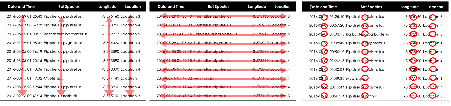
In Table 2.20 the is_unique(Species, DateTime) rule shows 6 fails in the statics data; to view these fails the violating function is used. Table 2.21 lists the fails in the statics data allowing the discrepancies in the data to be judged; although here the date/time and species is a duplication the Description’s are different (and therefore not a duplication). A better rule too use would be validator(is_unique(Description, Species, DateTime)).

Show the code

rule <- validator(is_unique(Species, DateTime))
out <- confront(statics, rule)

violating(statics, out) %>% 
  flextable() %>% 
  autofit() %>% 
    bold(part = "header") %>% 
    bg(bg = "black", part = "header") %>% 
    color(color = "white", part = "header") %>% 
    align(j = 1, align = "center", part = "header")

Table 2.21: Failed rows in the statics data

Description	DateTime	Species	Longitude	Latitude
Static 2	2016-07-30 23:16:59	Pipistrellus pipistrellus	-3.592583	50.33323
Static 4	2016-07-30 23:16:59	Pipistrellus pipistrellus	-3.591848	50.33130
Static 2	2016-08-04 22:12:36	Pipistrellus pipistrellus	-3.592583	50.33323
Static 4	2016-08-04 22:12:36	Pipistrellus pipistrellus	-3.591748	50.33136
Static 4	2016-08-25 22:08:10	Pipistrellus pipistrellus	-3.591738	50.33133
Static 5	2016-08-25 22:08:10	Pipistrellus pipistrellus	-3.590958	50.33105

Leo Tolstoy, opening lines of Anna Karenina (1873)↩︎
Hadley Wickham, author of many r packages expressing his view on Tidy Data (2014)↩︎
the standard is recommended by .gov.ukhttps://www.gov.uk/government/publications/open-standards-for-government/date-times-and-time-stamps-standard ↩︎
a full list of time zones can be found here https://en.wikipedia.org/wiki/List_of_tz_database_time_zones ↩︎
https://www.iczn.org/the-code/the-international-code-of-zoological-nomenclature/the-code-online/↩︎
Simmons, N.B. and A.L. Cirranello. 2023. Bat Species of the World: A taxonomic and geographic database. Version 1.3. Accessed on 03/14/2023.↩︎
https://en.wikipedia.org/wiki/World_Geodetic_System ↩︎
Adapted from EcoBat’s naming convention.↩︎